11 CMB mapmaking
Mapmaking, Noise, Time-ordered data
11 CMB mapmaking
11.1 The “naïve physicist”
The “naïve physicist” looks at this and says, “it is simple to reconstruct the CMB maps. Wherever the telescope is pointing to, we can simply average down the signal to the corresponding pixel.”
Except that it would not work, take a look at fig. 11.1:
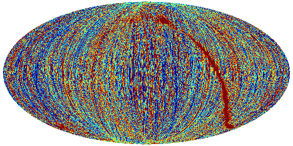
We can see visible vertical stripes here. These stripes will appear in the scanning directions because of the infamous \(1/f\) noise. The high amplitude, long time-scale noise is manifest in the next scanning line which now has a vastly different amplitude.
No wonder this is literally called naïve mapmaker.
11.2 The “naïve mathematician”
The “naïve mathematician” looks at eq. (10.1) and says, “wait a minute, I recognize this, this is just a standard linear regression problem, and we can write down the solution immediately by Generalized Least Squares (GLS).”
Indeed, by GLS, we know the solution to eq. (10.1) is2
\[\begin{align} N_{tt'} &= \left\langle n_t n_{t'} \right\rangle \nonumber \\ W_{pp'} &= P_{pt}^T N^{-1}_{tt'} P_{t'p'} \nonumber \\ \hat{m}_p &= W^{-1}_{pp'} P_{p't}^T N^{-1}_{tt'} d_{t'} \label{eq:map_estimator} \tag{11.1}\\ \text{Cov}(\hat{m}) &= W^{-1} \label{eq:map_covariance} \tag{11.2}\end{align}\]
Moreover, it can be shown that this solution is unbiased, and lossless in the sense that the Fisher information matrix with respect to the input parameters is preserved.
This is called maximal likelihood mapmaker, which is one example of optimal mapmakers that are lossless.
Indeed, this has been the mapmaker used in CMB experiments such as COBE (1990s) in the beginning. But as pointed out by Borrill,3 this has been computationally prohibitive for about 2 decades, because of the \(O(N_p^3)\) behavior of the algorithm involved in eq. 11.1 & 11.2.4
Today, a minority of CMB experiments still use this to solve for the map, but not the covariance. Hence their mapmaking is unbiased, but not lossless.
11.3 Naïve meeting naïve becomes not so naïve
One day the naïve physicist met the naïve mathematician, and they realized when the noise is uncorrelated white noise, then the naïve mapmaker is the optimal mapmaker.
But we have seen that the noise is far from white. We could, however, cheat and make it white.
The trick is to high-pass-filter our data to remove excessive low frequency noise. Then, as we have seen earlier, CRHWP modulation already makes the noise quite white to begin with.
But now we have a new problem, since we filtered our data, the map is now biased. And in practice, we typically have thrown away on the order of dozens of percent of information which is the cost to pay for this naïveness.
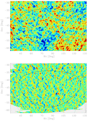
Fig. 11.2 shows us an example of high-pass filtering, we can see that the biased map below has much less large scale structure than the original input above. While the map is biased, its effect can be corrected in the power-spectrum domain via a method called MASTER devised in the same paper.
The tradeoff for the lossy mapmaking is now we have superior computational requirement. The naïve mapmaker, as we are simply binning the data, is a streaming algorithm, it has \(O(N_t)\) time complexity, and is embarrassingly parallel.
For example, this is the mapmaker of choice in the POLARBEAR experiment.
11.4 Unbiased mapmaking
But unbiased mapmaking is desirable if it is achievable. At the very least it is a cost tradeoff between data and computational time. To illustrate, it might be cheaper to build more detectors for ground-based experiments, but for satellite-based experiments, we definitely want to squeeze the last bit of information from the data. Not to mention unbiased maps can provide useful information within and beyond the CMB communities.
There are many unbiased mapmakers with different iterative solutions, examples are one used in a subset of POLARBEAR analysis,6 and the Madam mapmaker7 used in Planck analysis and will be used in many future CMB experiments including LiteBIRD.
They are often solving the mapmaking equation iteratively to achieve a lower time complexity, therefore they are unbiased and often asymptotically optimal.
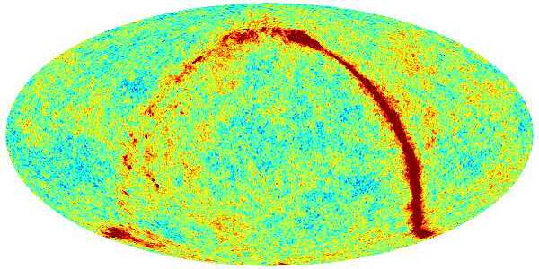
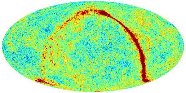
From the example of Madam mapmaker in fig. 11.3 & fig. 11.4, we can see that the two are very similar, meaning that the destriped map successfully recovers the noiseless map, comparing to the visible stripes in fig. 11.1.
Footnotes
Keihänen et al., “Making Cosmic Microwave Background Temperature and Polarization Maps with MADAM”.↩︎
How may \(N_{tt'}\) be estimated? In the framework of GLS, it is part of the model. That is, it is assumed to be a known quantity. In practice, one needs to build a model to describe the noise properties and then estimate the parameters of the noise model using the data. Note that in CMB observations, the signal is so faint that the TOD is dominated by the noise. In the special case that the noise model is uncorrelated white noise, one can simply estimate the noise variance using FFT on the TOD utilizing this fact. Incidentally, this technique is used in POLARBEAR. See Keihänen et al., “Making Cosmic Microwave Background Temperature and Polarization Maps with MADAM” for another assumption and technique to model and estimate the noise covariance.↩︎
“The Challenge of Data Analysis for Future CMB Observations,” 1999.↩︎
Actual time complexity is \(O(N_p^3)\) with a larger prefactor involving multiple Cholesky decompositions in later steps. See Borrill, for details.↩︎
Hivon et al., “MASTER of the Cosmic Microwave Background Anisotropy Power Spectrum”.↩︎
Poletti et al., “Making Maps of Cosmic Microwave Background Polarization for B-Mode Studies”.↩︎
Keihänen et al., “Making Cosmic Microwave Background Temperature and Polarization Maps with MADAM”.↩︎
Keihänen et al., “Making Cosmic Microwave Background Temperature and Polarization Maps with MADAM”.↩︎