27 Analytical methods
POLARBEAR, Pseudo-spectra and MASTER, Power spectra, Masks and apodization, Filtering, Noise, Simulations
27 Analytical methods
We will go through the main analytical methods involved here. The general framework is the same with previous B-mode papers from POLARBEAR.1 The basic approach will be outlined here, with more details provided whenever they differ.
27.1 Cross-pseudo-power-spectra calculation
We briefly outlined the cross-pseudo-power-spectra in sec. 21.3. Equation-wise, it is well-documented in previous POLARBEAR publications on B-mode. It is based on Hinshaw et al.2
We mentioned earlier 38 map-bundles were formed. Each of them amounts to about 10 days’ worth of observations, and each forms a complete map of the observed patch of sky.
This cross-map approach assumes that each map-bundle is an independent observation of the sky. So the cross-pseudo-power-spectra would be noise-free and bias-free. The validity of the assumption is from empirical knowledge that the correlations in the TOD have a timescale of around \({20\,\mathrm{min}}\), and from empirical studies including the null-test suite. Hence, this estimator provides a signal-only estimation.
The noise pseudo-power-spectra can be estimated by first calculating the pseudo-power-spectra of the full map (that is coadded from all 38 map-bundles), often called the auto-power-spectra, and subtracting the signal-only estimate from previous step.
27.2 Smoothing and tapering of the maps
As the estimate of \(E\)-mode and \(B\)-mode involves 2nd order derivatives3, we need to make sure the input maps are at least twice differentiable. Also, at the edge of the map, derivatives can be problematic. Hence, a tapering is usually done to ensure gradual transition to zero. Finally, in the calculation of pseudo-power-spectra, we would want the region with a lower level of noise to be weighted more heavily to reduce the resultant error-bar. Naturally, as we already have the weight map4, it is used for this purpose.
Putting all together, the weight map will be smoothed, tapered—the product of which is often called the weight-mask or simply mask—and will be multiplied to the map before performing pseudo-power-spectra estimation in the previous section.
In previous POLARBEAR B-mode analyses, a Hamming window with a scale of \({0.53^\circ}\) is used to smooth the map, and a \(C^2\)-tapering of \({0.5^\circ}\) wide is performed at the edge. These weight maps are calculated per map within the map-bundles.
In this analysis, a Gaussian blur of \({3.3013338110314874'}\)5 is used to smooth the map, and a \(C^\infty\)-tapering with a scale of \({1^\circ}\) is applied at the edge.
27.3 Monte Carlo Apodized Spherical Transform Estimator (MASTER)
MASTER is “a fast and accurate method for estimation of the cosmic microwave background (CMB) anisotropy angular power spectrum”6.
This is the central concept that enables the naïve mapmaker that biases (filtering) is allowed but will be de-biased in the power-spectra domain. And the effect of the weight mask from the previous section will also be accounted for. Mathematically,
\[\tilde{C}_\ell = \sum_{\ell'} M_{\ell \ell'} F_{\ell'} B^2_{\ell'} C_{\ell'}\]
Here, \(C\) is the original, un-biased (cross-)power-spectrum. \(B\) is the beam profile, \(F\) is the filter transfer function, and \(M\) is the mode-coupling matrices. \(\tilde{C}\) is the pseudo-(cross-)power-spectra that we can measure in sec. 27.1.
The beam is measured in previous steps7 and is known at this stage. Mode-coupling matrices account for the fact that multiplying a weight-mask would change the resultant power-spectra and is the topic later in sec. 27.4 and can be calculated analytically given the weight-mask.
Had we known the filter transfer function \(F\), we could have used that to invert the formula and would have obtained an unbiased estimate of \(C\).
The key idea in using this equation is that we can perform Monte Carlo (MC) simulations to estimate \(F\). Specifically, we can run MC simulations that replicate the actual experiment including any filtering effects, resulting in
\[\tilde{C}^\text{MC}_\ell = \sum_{\ell'} M_{\ell \ell'} F_{\ell'} B^2_{\ell'} C^\text{MC}_{\ell'}\tag{27.1}\]
Here, \(C^\text{MC}\) is a known input, \(\tilde{C}^\text{MC}\) can be calculated as outlined in sec. 27.1. Hence we can solve this equation and obtain an estimate of \(F\).
In fact, since there are \(E \rightarrow B\) leakage and vice versa, we can perform different MC simulations with one set of maps having only \(T, E\) signals, and another set having only \(T, B\). This allows us to estimate \(F^{EE \rightarrow BB}, F^{BB \rightarrow EE}\) in addition to \(F^{TT \rightarrow TT}, F^{EE \rightarrow EE}, F^{BB \rightarrow BB}\).
Now, the devil is in the details. How do we invert eq. (27.1)? Note that the mode-coupling matrices have a very high condition number unless we have close to full-sky coverage8. Inverting it numerically is technically possible but the resultant \(F\) would have huge numerical error making it not usable.
Hivon et al.9 has mentioned an iterative approach to estimate \(F\). This approach inherently depends on the number-of-iterations parameter \(n_\text{iter}\). Note that when \(n_\text{iter} \rightarrow \infty\) it should recover the \(F\) with high numerical error, as the iterative approach is solving the inverse matrix problem iteratively. \(n_\text{iter}\) has to be chosen carefully. Hivon et al.10 chose \(n_\text{iter} = 1\) for BOOMERANG, and The POLARBEAR Collaboration et al.11 chose \(n_\text{iter} = 10\) for POLARBEAR’s small-patch experiment.
Below we will describe another method that has no such arbitrary parameter for the numerical solution.
Modified MASTER
The key idea is to move the term \(F\) to the left,
\[\tilde{C}'_\ell = \sum_{\ell'} F'_\ell M_{\ell \ell'} B^2_{\ell'} C_{\ell'}.\tag{27.2}\]
The prescription here is clearly wrong. The filter transfer function captures the effect of the filtering performed on the TOD. The mode-coupling effect happens at a later stage when calculating the pseudo-(cross-)power-spectra. So only the order prescribed in MASTER is correct.
Analytically, if \(M\) is diagonal or \(F\) is a constant, the modified MASTER and the original MASTER are the same. We know that \(M\) is close to diagonal (in the sense that main diagonal is dominant in magnitude) and \(F\) is slowly varying across \(\ell\).
Empirically, it should be mentioned that the estimate of \(F\) is never exact here, because it is estimated using MC simulations, and because it is numerically unstable to construct \(F\) exactly.
So phenomenologically, as long as the error made is small, eq. (27.2) should be ok.
Note that if we define
\[\tilde{C}''_\ell = \sum_{\ell'} M_{\ell \ell'} F'_{\ell'} B^2_{\ell'} C_{\ell'}\tag{27.3}\]
Then
\[\tilde{C}'_\ell - \tilde{C}''_\ell = \sum_{\ell'} \left( F'_{\ell} M_{\ell \ell'} - M_{\ell \ell'} F'_{\ell'} \right) B^2_{\ell'} C_{\ell'}\]
So the difference is roughly speaking a commutator between \(M, F\).
To find out the error made when using the modified MASTER, we can use MC simulations eq. (27.1). Note that in this equation, both \(\tilde{C}\) and \(C\) are known. We can then use eq. (27.2) to estimate \(F'\), plug that in eq. (27.3), and calculate the quantity
\[\frac{\tilde{C}''_\ell - \tilde{C}_\ell}{\tilde{C}_\ell}.\]
This represents the relative error made in terms of the resultant pseudo-power-spectra had we known the true \(F\) but used the modified MASTER to estimate \(F'\) instead.
Estimating this relative error in the pseudo-power-spectra cases of \(TT, EE, BB\), which is shown in fig. 27.1, fig. 27.2, fig. 27.3 using 128 MC simulations, we see that the relative error is small (RMS at \(\sim {0.5\,\%}\) across \(600 \leq \ell \leq 3000\)) and unbiased. As the bin-width used in a later step is 100, the error would be much smaller.
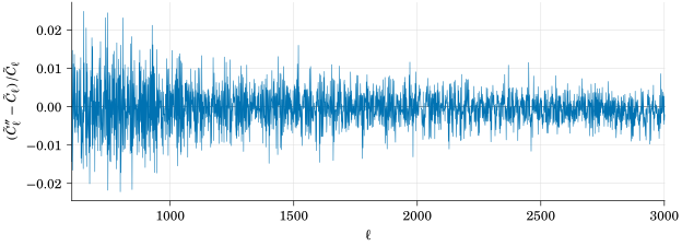
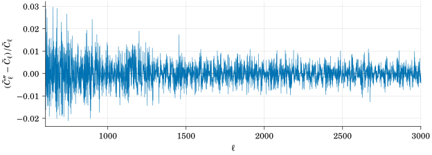
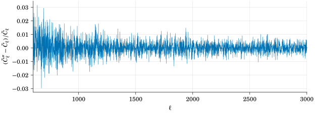
Not only that, empirically, I find that this relative error is roughly inversely proportional to \(F'\). Since \(0 < F \leq 1\), empirically as long as \(F'\) is not close to zero12, the approximation performed by the modified MASTER should be small.
Note that the relative error mentioned here is comparing between modified MASTER and the original MASTER, in my pipeline I consistently always use the modified MASTER throughout the pipelines so the actual error made should be even smaller.
To conclude, we find that the modified MASTER is parameter-free requiring no tuning, the error made is negligible, and is good enough phenomenologically in this particular analysis.
Finally, it should be noted that this modified MASTER may be used elsewhere. It may have been mentioned in casual conversations with other CMB scientists. The justification here may be new in the sense that it is shown here explicitly why we can do this.
27.4 Mode-coupling calculations
We will briefly go through how the mode-coupling matrices are estimated.
First, the mode-coupling matrix is often written as \(M^{XYXY}\), or \(M^{XY \rightarrow XY}\), representing the mode-coupling matrix from the \(XY\) power-spectra to the \(XY\) pseudo-power-spectra.
\(XY\) can be any cross-spectra \(TT, EE, BB, TE, TB, EB\).
For the \(TT\) case, Hivon et al.13 has derived it in the appendix. For the rest which includes polarizations, Miller14 documented them in an internally circulated document, and implemented it in AnalysisBackend. In these equations, the B-mode is assumed to be constructed by the pure B-mode estimator.15
Later, I found some problems in AnalysisBackend regarding the mode-coupling matrix calculations.
First, there is a bug that in the case of \(EB\), the pure \(B\)-mode estimator is not used. Second, there are various numerical problems in the calculation that the matrices deviate from actual values when it is far away from the main diagonal.
The mode-coupling matrix code is completely rewritten to fix this, in addition to making it run much faster as explained in chapter 25. This module is released in TAIL.
There is another subtlety related to the calculation of mode-coupling matrices. In the previous pipelines of POLARBEAR \(B\)-mode analysis, each map-bundle uses their own weight-mask, which implies that the mode-coupling matrix calculated here is not correct (as the analytical formula assumes all share the same weight-mask.) Phenomenologically, using MC simulations, previous pipelines can recover unbiased power-spectra empirically. Alternatively, we can use a single weight-mask (constructed using the fully coadded map.) The disadvantage of this approach is that the weight-mask applied is less than optimal, and therefore potentially reducing sensitivity in the end. Both approaches have been compared in this study, and no major differences between them are found. In the end, the latter approach is taken as it is better safe (less than optimal) than sorry (wrong mode-coupling matrices applied.)
27.5 Zero padding of the map for the calculation of the power-spectra
In the calculation of the pseudo-(cross-)power-spectra in sec. 27.1, because an FFT is needed to first transform the map into frequency domain, zero-padding is required as FFT assumes periodicity.
However, how much zero-padding is needed? If we simply estimate from eq. (23.1), as the lowest \(\ell\) here is \(600\), it corresponds to around \({18'}\) on both ends. This amounts to only \(9\) pixels wide in \({2'}\) resolution.
However, as Kuo et al.16 said,
For a strictly stationary process this is not a problem since the correlation usually vanishes after a sufficiently long time lag. For piecewise stationary processes, a straightforward application of FFT produces false correlation for lag \(> n/2\), where \(n\) is the number of elements. This can be prevented by zero padding.
So a \(2\times\) zero-padding is recommended when calculating the pseudo-power-spectra.
The effects of zero-padding between \(1.3\times\) and \(2\times\) are compared in this study and negligible differences are found from simulations. However, as a caution, we still follow the standard practice of having \(2\times\) zero-padding in the final analysis.
27.6 Noise
Noise estimate is used in 2 places, one in the coadd pipeline where the noise is used to determine the weight, and another when noise is injected in the simulations to mimic the real observations where the statistical fluctuations in the resultant power-spectra are used to estimate the statistical error-bar of the power-spectra.
There are 2 noise pipelines. In the first one, we assume an uncorrelated white noise model, and estimate them in the TOD. This is always the noise model used to construct the weight-maps. Optionally, this white noise model is also used in the simulation to simulate noisy observations.
Another noise pipeline is called sign-flipped noise. Assuming the maps containing signal and noise terms only, if we randomly assign a sign in the coadd process to the maps, then the coadded map should on average contain no signal and only have noise.
These 2 noise pipelines are compared, and they are found to be in general agreement in \(N^{EE}, N^{BB}\), as the assumption of uncorrelated white noise is very good there because of the CRHWP modulation away from the \(1/f\) noise17. This is not true for the temperature maps and its noise power-spectra \(N^{TT}\) simply because of the \(1/f\) noise.
As explained before, less than optimal construction of the weight-maps only results in less than optimal (bigger error-bar) but usable resultant maps.
To obtain a realistic error-bar in simulations including the intensity map, we opt for the sign-flip noise. With this realistic estimate of statistical errors, we shall soon see we can pass the null-test suite even if we include the temperature-related power-spectra (including \(TT, TE, TB\)) for the first time in POLARBEAR. These power-spectra are used for absolute gain calibration later.
Footnotes
The POLARBEAR Collaboration et al., “A Measurement of the Cosmic Microwave Background B-Mode Polarization Power Spectrum at Sub-Degree Scales with POLARBEAR”; The POLARBEAR Collaboration et al., “A Measurement of the Cosmic Microwave Background B-Mode Polarization Power Spectrum at Subdegree Scales from Two Years of POLARBEAR Data”; The POLARBEAR Collaboration et al., “A Measurement of the Degree-Scale CMB B-Mode Angular Power Spectrum with POLARBEAR”.↩︎
“First‐Year Wilkinson Microwave Anisotropy Probe ( WMAP ) Observations”.↩︎
To recall, the weight map is precision—the inverse of the variance at each pixel on the map.↩︎
The number is chosen so that this Gaussian window is minimally different from the Hamming window above.↩︎
Hivon et al., “MASTER of the Cosmic Microwave Background Anisotropy Power Spectrum”.↩︎
This can be understood by observing in the limit of full-sky coverage, \(M \rightarrow I\) the identity matrix.↩︎
“MASTER of the Cosmic Microwave Background Anisotropy Power Spectrum”.↩︎
“MASTER of the Cosmic Microwave Background Anisotropy Power Spectrum”.↩︎
“A Measurement of the Cosmic Microwave Background B-Mode Polarization Power Spectrum at Sub-Degree Scales with POLARBEAR”.↩︎
This is a region that the de-biased power-spectra would have close to infinite error which is not usable anyway.↩︎
“MASTER of the Cosmic Microwave Background Anisotropy Power Spectrum”.↩︎
Smith, “Pseudo- C ℓ Estimators Which Do Not Mix E and B Modes”.↩︎
“High‐Resolution Observations of the Cosmic Microwave Background Power Spectrum with ACBAR”.↩︎
The POLARBEAR Collaboration et al., “A Measurement of the Cosmic Microwave Background B-Mode Polarization Power Spectrum at Sub-Degree Scales with POLARBEAR” further compared between correlated and uncorrelated white noise models and found them to be consistent.↩︎