36 Crosstalk systematics simulations with hardware based mitigation
LiteBIRD, Crosstalk, Systematics, Detectors and readout, Half-wave plate, Simulations
36 Crosstalk systematics simulations with hardware based mitigation
36.1 Introduction
This section puts everything together and demonstrates the simulation of the crosstalk systematics using the LiteBIRD Instrument Model (IMo) v1 as an example.
Terminologies & conventions of detectors
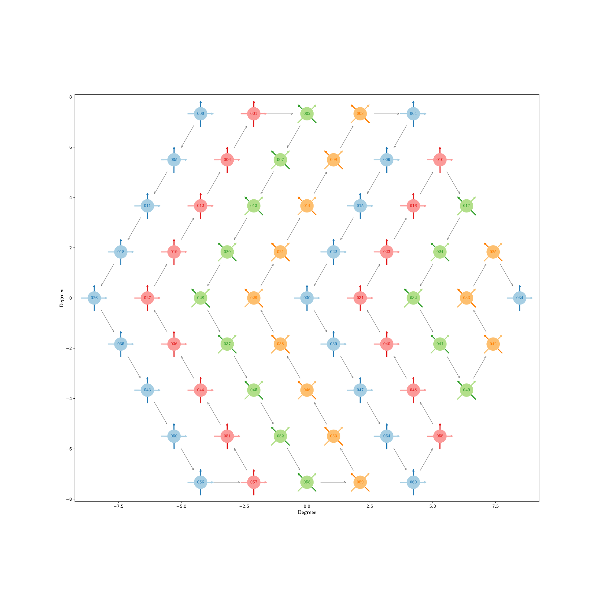
Fig. 36.1 shows an example focal plane using the MFT central wafer at \({140\,G\mathrm{Hz}}\).
| \(T\) | \(B\) | |
|---|---|---|
| \(Q\) | \({0^\circ}\) | \({90^\circ}\) |
| \(U\) | \({45^\circ}\) | \({135^\circ}\) |
| color | light | dark |
| \(A\) | \(B\) | |
|---|---|---|
| \(Q\) | Blue | Red |
| \(U\) | Green | Orange |
\(Q\) detectors are represented by arrows at \({0^\circ}, {90^\circ}\), and \(U\) detectors are represented by arrows at \({45^\circ}, {135^\circ}\). They are color-coded in brightness as summarized in tbl. 36.1. Then there are 2 kinds of detector handedness, where one is a mirror image of another. They are simply named \(A, B\). The 4 combinations of \(Q, U\) and \(A, B\) are color-coded according to tbl. 36.2. Hence, the colors blue, red, green, orange correspond to QA, QB, UA, UB.
Also note that \(n\)-th nearest neighbor can be in focal plane (angular distance) or in SQUID (frequency) depending on the context.
36.2 2-detectors simulations
Decomposition of crosstalk matrix
First, a constant crosstalk matrix with only non-zero elements in the nearest neighbor (in SQUID) is considered. In the limit of infinitely long SQUID, it can be decomposed in a superposition of 2-detectors crosstalk matrix like this:
\[\begin{bmatrix} 1/2 & x & 0 & \dots \\ x & 1/2 & 0 & \dots \\ 0 & 0 & 0 & \dots \\ \vdots & \vdots & \vdots & \ddots \\ \end{bmatrix} + \begin{bmatrix} 0 & 0 & 0 & \dots \\ 0 & 1/2 & x & \dots \\ 0 & x & 1/2 & \dots \\ \vdots & \vdots & \vdots & \ddots \\ \end{bmatrix} + \dots = \begin{bmatrix} 1/2 & x & 0 & 0 & \dots & \dots \\ x & 1 & x & 0 & \dots & \dots \\ 0 & x & 1 & x & \dots & \dots \\ 0 & 0 & x & 1 & \ddots & \dots \\ \vdots & \vdots & \vdots & \ddots & \ddots & x \\ \vdots & \vdots & \vdots & 0 & x & 1/2 \\ \end{bmatrix}\]
The decomposition is exact in TOD. It should be approximately true in map-domain and eventually power-spectra-domain as well if \(x \ll 1\).
Moreover, in a realistic crosstalk matrix simulated from SQUID, it is approximately true that the next nearest neighbors (in SQUID) are of lower orders, whereas the nearest neighbor crosstalk is of the same order of magnitude. (See more in Montgomery1 or below.)
This means that if the 2-detector case is understood, it can be generalized to a long SQUID approximately.
2-detectors simulation results
Below are the systematic effects of a pair of detectors in \(\frac{C_\ell^\text{crosstalk}}{C_\ell}\),
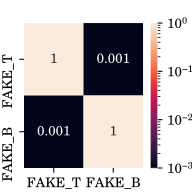
- Using IMO v1.0 parameters,
- Modified from the central pixel of MFT at \({140\,G\mathrm{Hz}}\),
- Scanning from a
synfastinput map using Planck 2018 best-fit ΛCDM cosmology with 183 days of observations, - At an angular distance of \({2.114^\circ}\) (corresponding to the mean lattice angular distance of the MFT hexagonal wafer),
- varying the polarization angles of the 1st and 2nd detectors.
Below, 1st number is 1st detector polarization angle, last number is 2nd detector polarization angle.
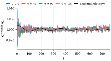
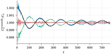
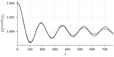
Figure 36.3: 2-detectors crosstalk systematics expressed as \(\frac{C_\ell^\text{crosstalk}}{C_\ell}\). The legend in (a) applies to all panels.
fig. 36.3 shows the result of the simulations, presented as a transfer function of the power-spectra. These can be compared to the analytic formula in sec. 34.3 shown in the plot. There is a high level of agreement, with the exception of damping towards high-\(\ell\), which is an effect similar to the PWF as the analytical model assumes a delta function, while in mapmaking, finite size pixels are used.
Lesson learnt—rule of thumb of wafer ordering
Combining the empirical simulation results and the analytical behavior expected from (34.11), the crosstalk systematics have minimal effects on the resultant \(EE, EB, BB\) power-spectra in these special cases,
- \(\theta = 0\), or
- for \(\alpha\) to be either
- \(\alpha = {45^\circ}\) or \({135^\circ} \rightarrow \frac{C_\ell^\text{crosstalk}}{C_\ell} = 0\)
- \(\frac{C_\ell^\text{crosstalk} (\alpha = {0^\circ})}{C_\ell} = -\frac{C_\ell^\text{crosstalk} (\alpha = {90^\circ})}{C_\ell}\)
Now, we can apply what we learnt in wafer & SQUID design using the following empirical rules. Design here means that given a wafer, there is a considerable degree of freedom in how to wire the detectors together (ordering in SQUID) and how to walk the wafer. Here is an empirical algorithm in doing so.
Corollary 2. Rule-of-thumb to design the wafer to minimize crosstalk systematics.
Walk within the same pixel first, as this has no bias (\(\theta = 0\)).
Then walk to the nearest neighbors on the focal plane (note that in a hexagonal wafer this always injects systematics at the same angular scale \(\theta\), but a rectangular one has 2 angular scales). This rule comes from limitations in how they can be wired physically.
Calculate \(\alpha\), the angle turned when walking from one pixel to another, following the following preferences:
Prefer \({45^\circ}\) or \({135^\circ}\), as (34.11) shows this has no bias up to 1st order2, otherwise,
if a pair has a rotation of \({0^\circ}\) (\(\cos 0 = 1\)), balance it by another pair that rotates by \({90^\circ}\) (\(\cos {90^\circ} = -1\)). Essentially, for the whole SQUID, \(\sum_i \cos (2 \alpha_i) = 0\) is desired as a rule of thumb3. If there are multiple angular scales in walking the focal plane (for example, in LFT), balance this for each angular scale individually.
36.3 Full wafer simulations—Realistic wafer simulation with the example of the central wafer of MFT at \({140\,G\mathrm{Hz}}\) with 2 SQUIDs each having 61 detectors
Wafer mockups
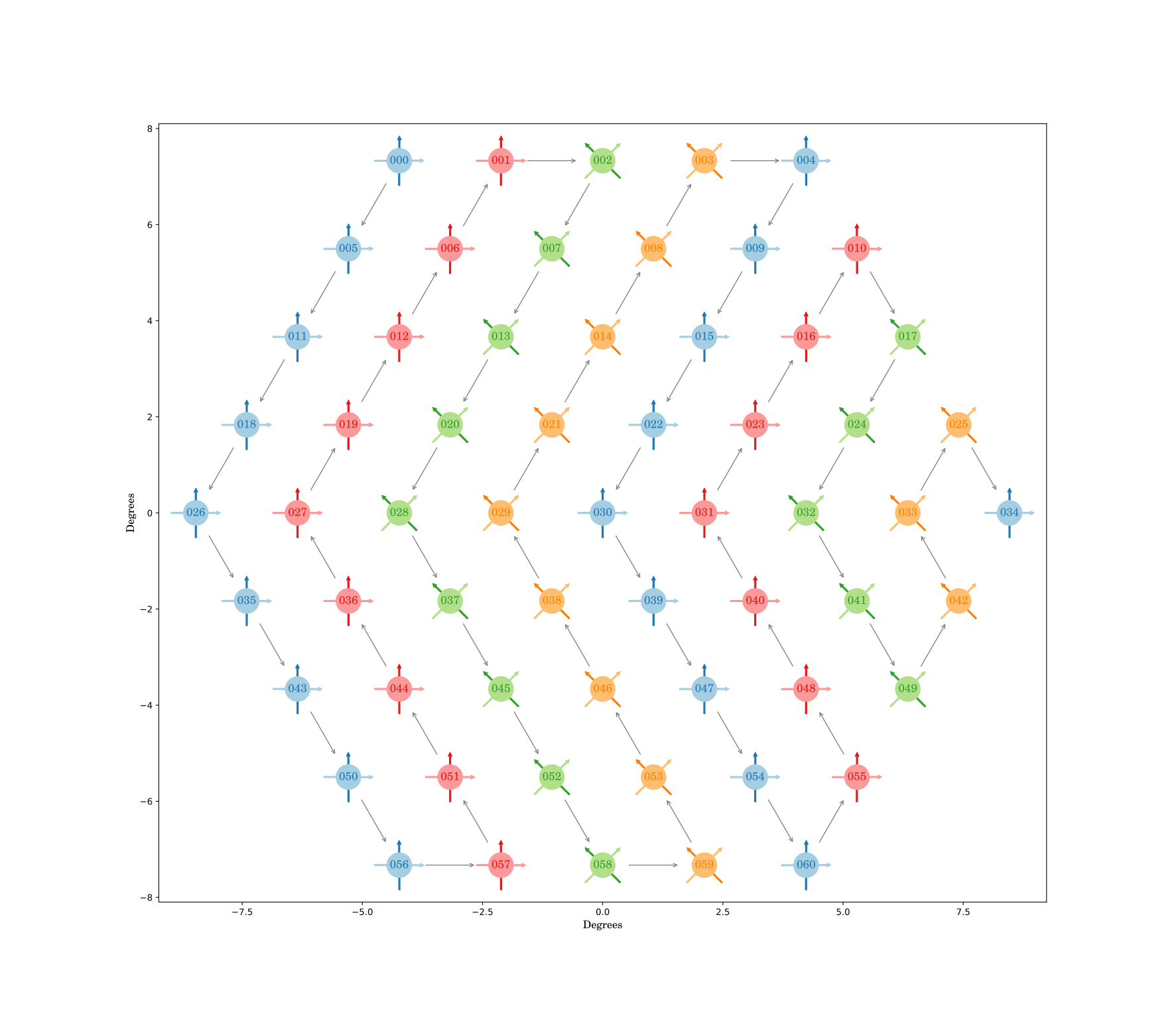
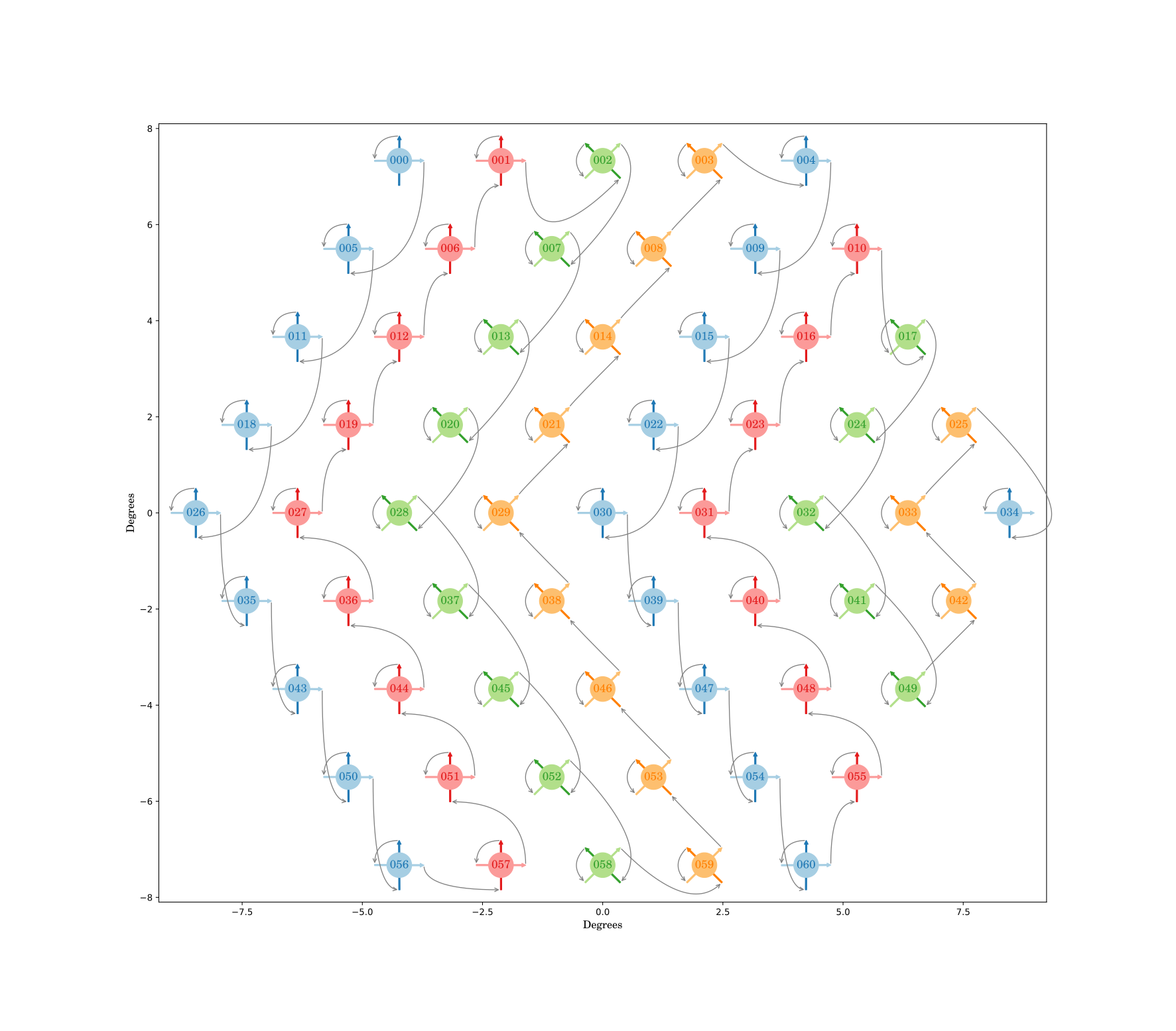
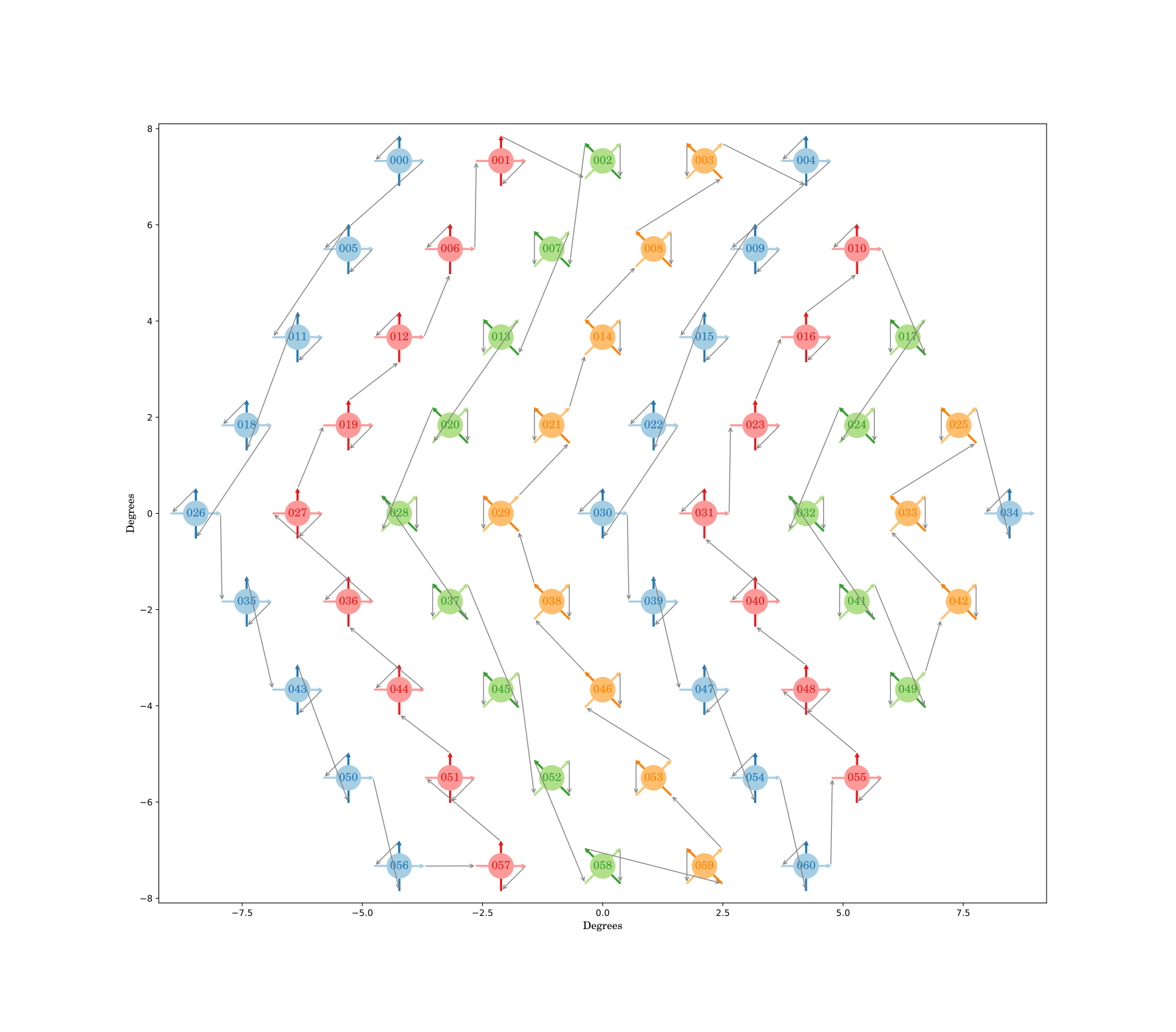
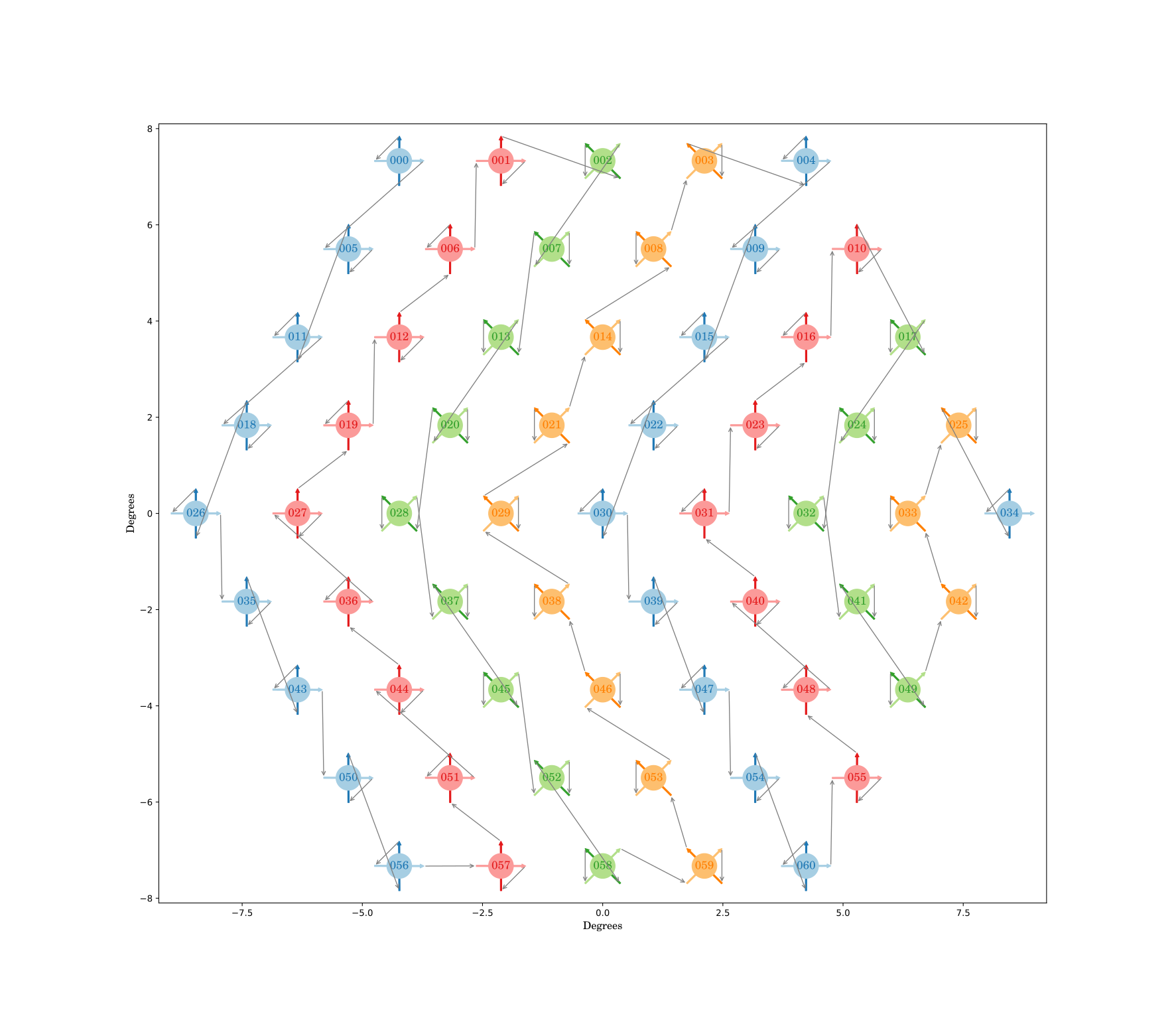
Figure 36.4: ArrowTopLeftFirst: a wafer design to walk the wafer. The top-left plot shows the ordering in pixel order only. The other 3 plots show the \(T\)/\(B\)-wiring explicitly, each with a different \(T\)/\(B\) ordering.
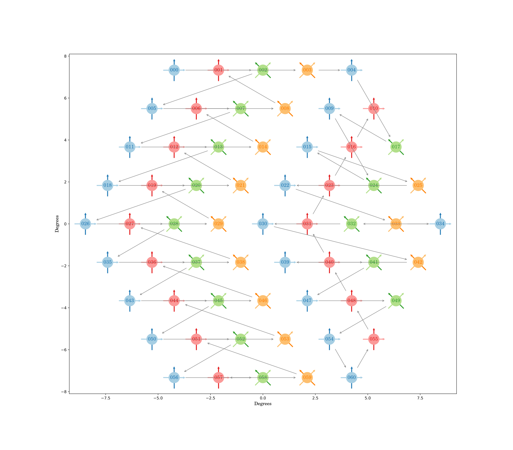
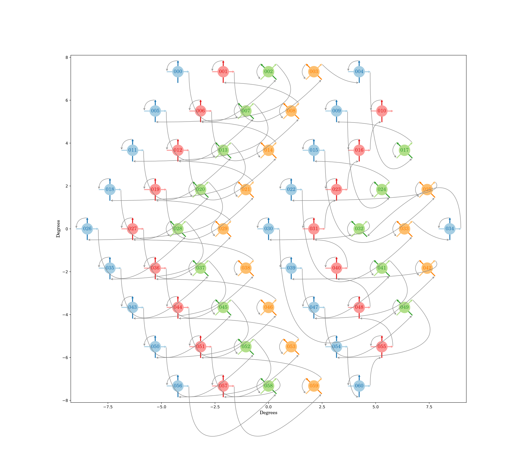
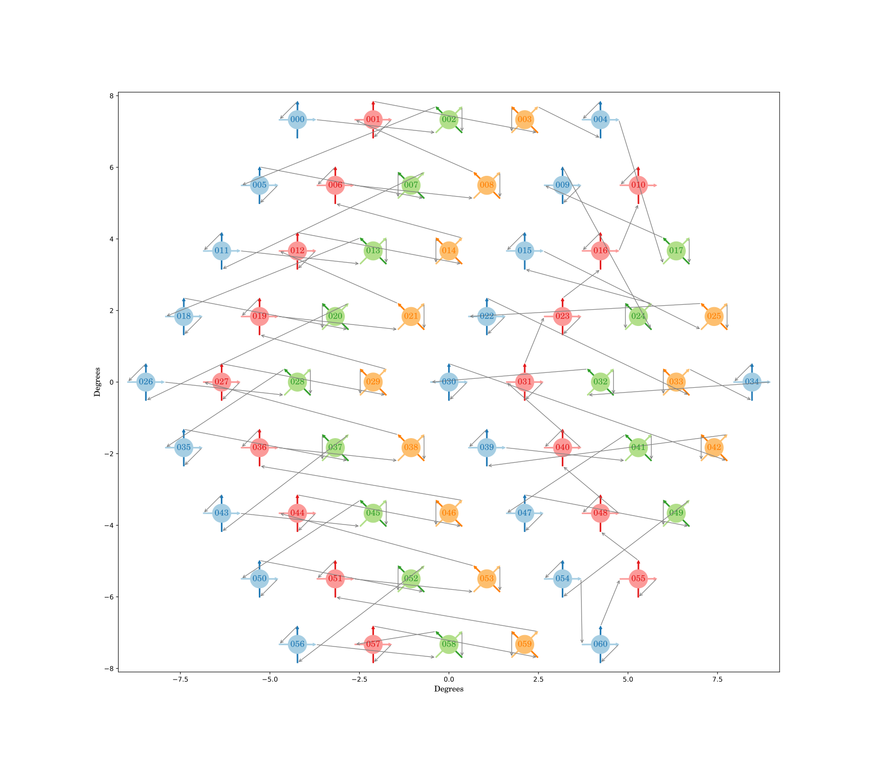
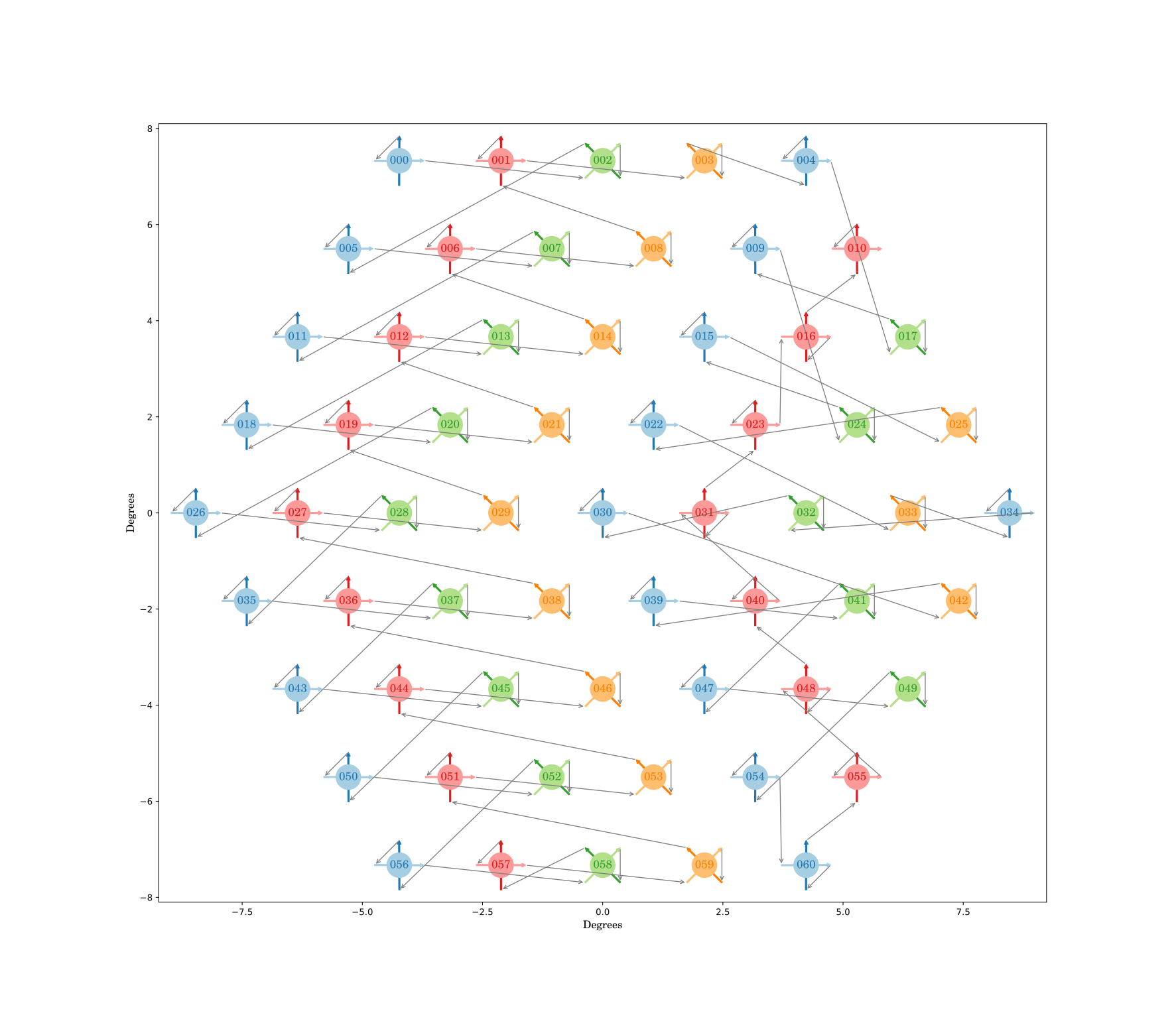
Figure 36.5: AlternateQU: a wafer design to walk the wafer. The top-left plot shows the ordering in pixel order only. The other 3 plots show the \(T\)/\(B\)-wiring explicitly, each with a different \(T\)/\(B\) ordering.
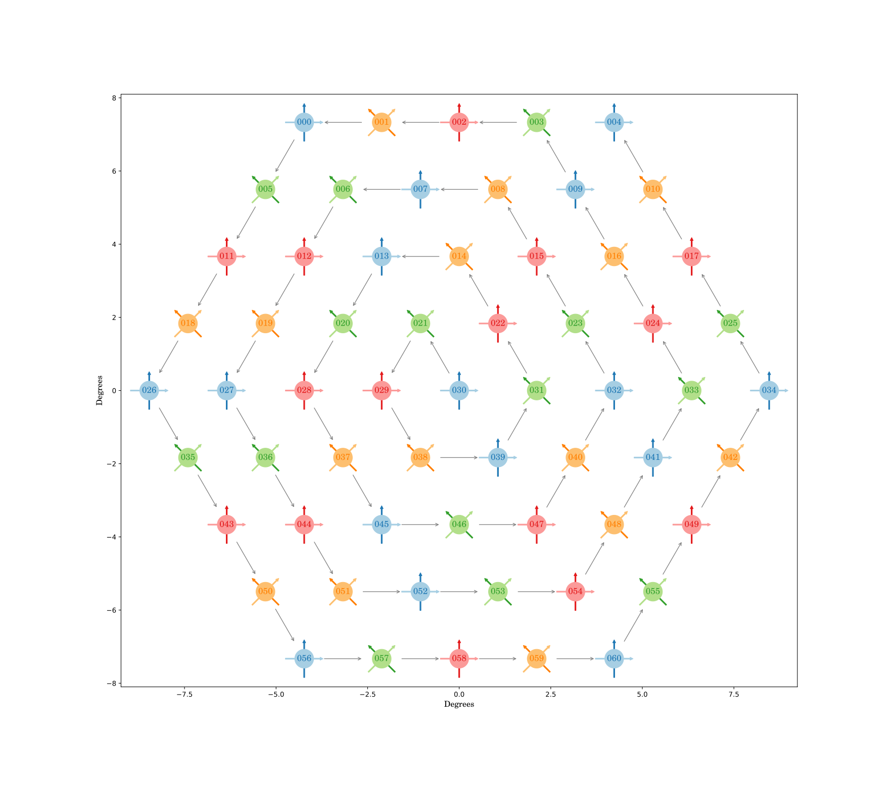
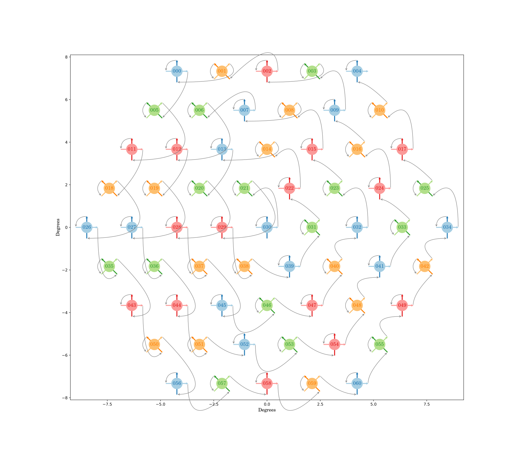
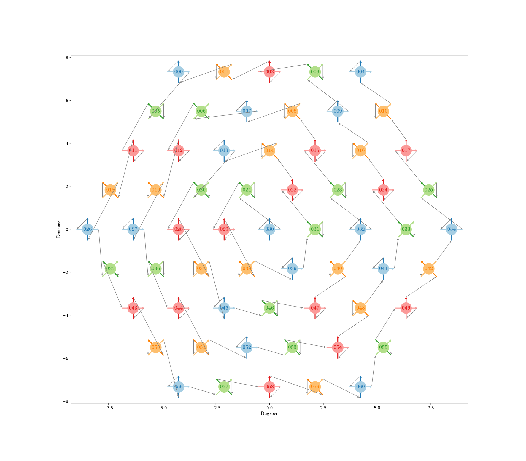
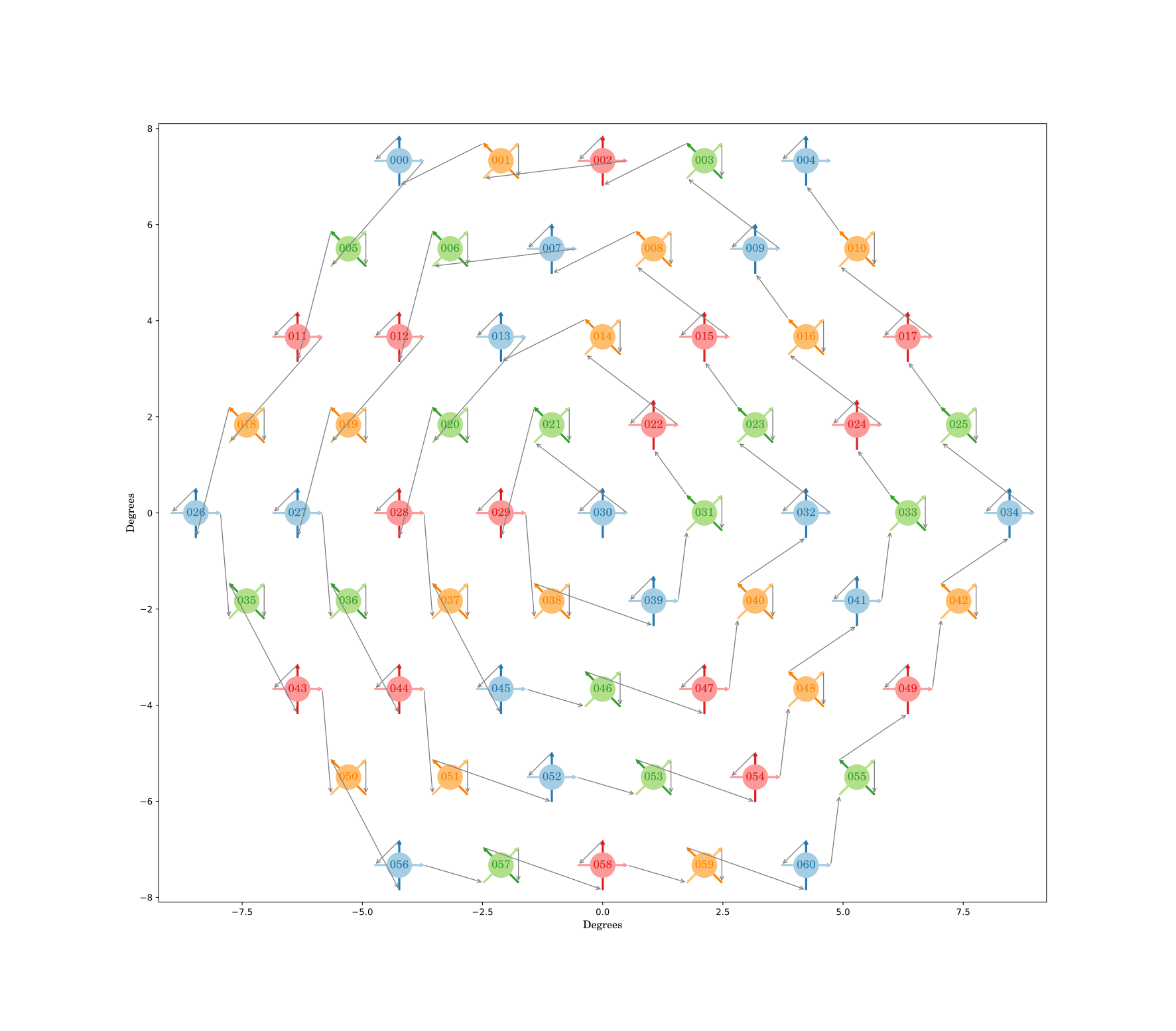
Figure 36.6: SpiralCounterclockwise_QUAB: a wafer design to walk the wafer. The top-left plot shows the ordering in pixel order only. The other 3 plots show the \(T\)/\(B\)-wiring explicitly, each with a different \(T\)/\(B\) ordering.
In fig. 36.4, fig. 36.5, fig. 36.6, we look at 3 different wafer mockups ArrowTopLeftFirst, AlternateQU, & SpiralCounterclockwise_QUAB.
In the first 2 cases, ArrowTopLeftFirst, AlternateQU, the IMO v1 MFT central wafer at \({140\,G\mathrm{Hz}}\) is taken as is.
In ArrowTopLeftFirst, it walks the focal plane by following the same QA line first, etc., that is, most of the walking across pixels happens at \({0^\circ}\) or \({90^\circ}\), this follows Corollary 2 2b.
In AlternateQU, when crossing between pixels, it tries to go from a \(Q\)-pixel to a \(U\)-pixel as much as possible. This follows Corollary 2 2a. Note that since the wafer has more Q-pixels than U-pixels, the last few detectors cannot fulfill this.
In the last case SpiralCounterclockwise_QUAB, the wafer is redesigned in a way that given a SQUID-ordering on the focal-plane, the ordering is alternated between \(Q\) and \(U\)-pixels. This follows Corollary 2 2a exactly by construction. Note that this has a considerable degree of freedom and the only requirement is that the numbers of \(Q\) and \(U\)-pixels are balanced.
“TB-alignment” represents when walking to the next detector, how to wire between the Top & Bottom detectors.
- normal
- It always walks from a Bottom detector to a Top detector in a new location.
- \(0T \rightarrow 0B \rightarrow 1T \rightarrow 1B \rightarrow 2T \rightarrow 2B \rightarrow 3T \rightarrow 3B \ldots\)
- This results in \(\sum_i \cos (2 \alpha_i)\) maximally negative.
- TB-anti-alignment
- It always walks from a Bottom detector to a Bottom detector in a new location, similarly for Top to Top.
- \(0T \rightarrow 0B \rightarrow 1B \rightarrow 1T \rightarrow 2T \rightarrow 2B \rightarrow 3B \rightarrow 3T \ldots\)
- This results in \(\sum_i \cos (2 \alpha_i)\) maximally positive.
- TB-alternate-anti-alignment
- It mixes the above 2 strategies alternatively.
- \(0T \rightarrow 0B \rightarrow 1B \rightarrow 1T \rightarrow 2B \rightarrow 2T \rightarrow 3T \rightarrow 3B \ldots\)
- This results in \(\sum_i \cos (2 \alpha_i) \approx 0\) by alternating between the 2.
These serve as examples. Other orderings following similar schemes are explored, which seem to indicate the general characteristics in the final power-spectra do not depend on the exact details of how they are ordered, as long as Corollary 2 is followed.
Full wafer simulation results
Similar to the 2-detectors case, but now with the wafer defined above, with 122 detectors and 4 days of observations (with a sky coverage around \(60–{70\,\%}\).)
For the crosstalk matrix, the following SQUID parameters are used, this is similar to the SPT-3G design,4 slightly modified for the LiteBIRD case provided by Joshua Montgomery, with \(L_\text{com}\) chosen with the expectation of using \({\text{µ}\mathrm{K}}\)-SQUID.
\[\begin{align*} R_\text{TES} &= {0.6\,\Omega} \\ r_s &= {0.3\,\Omega} \\ L &= {60\,\text{µ}\mathrm{H}} \\ L_\text{com} &= {9\,n\mathrm{H}} \\ f_\text{min} &= {1.69\,M\mathrm{Hz}} \\ f_\text{max} &= {5.49\,M\mathrm{Hz}} \end{align*}\]
with 68 detectors with SQUID frequencies spacing linearly between its min/max.
Then the highest 7 frequencies are removed to have a crosstalk matrix of 61 detectors, as shown in fig. 36.7.
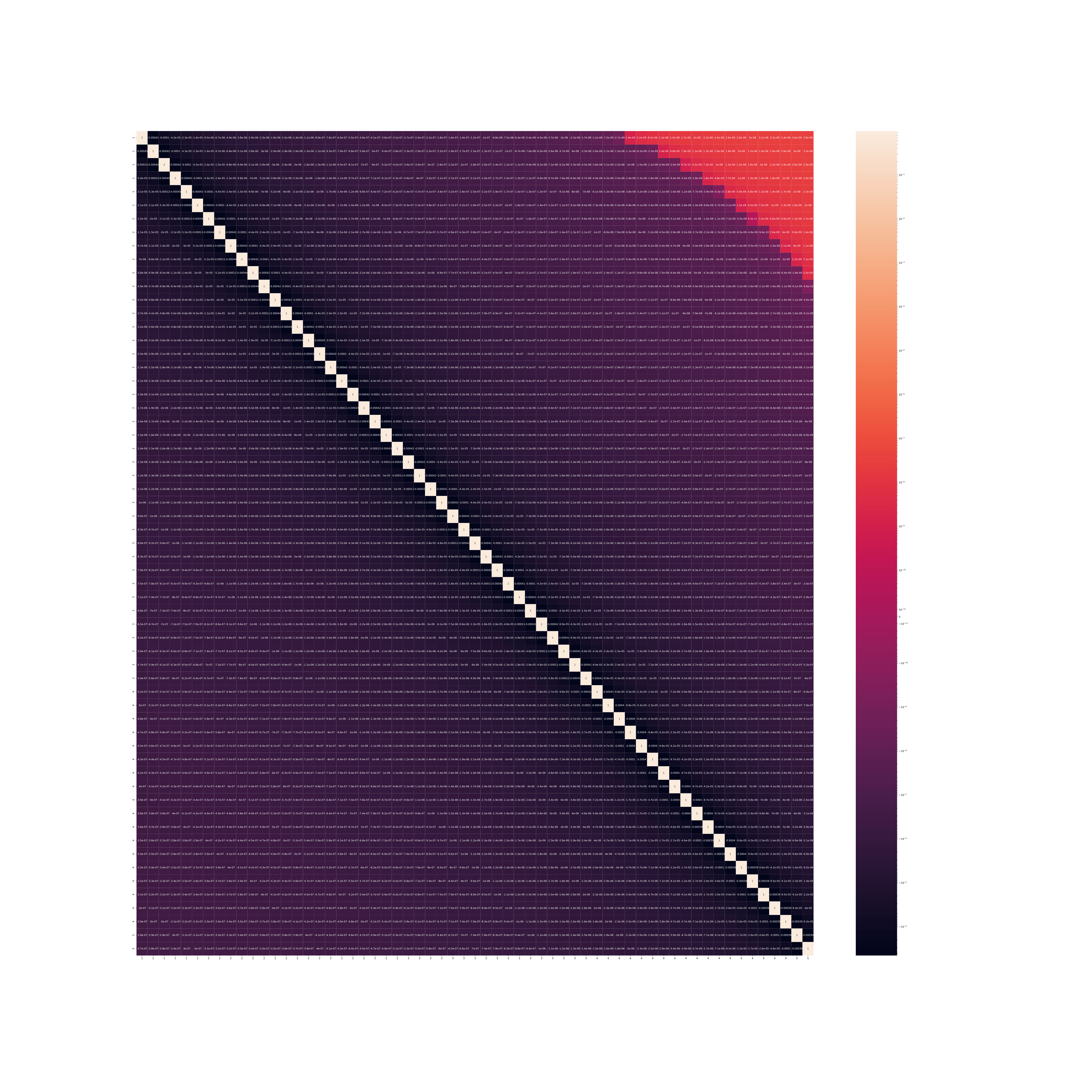
And 2 such SQUIDs are put in the focal plane in the previous sections. That is, the first 61 detectors belong to the 1st SQUID, the last 61 to the 2nd SQUID.
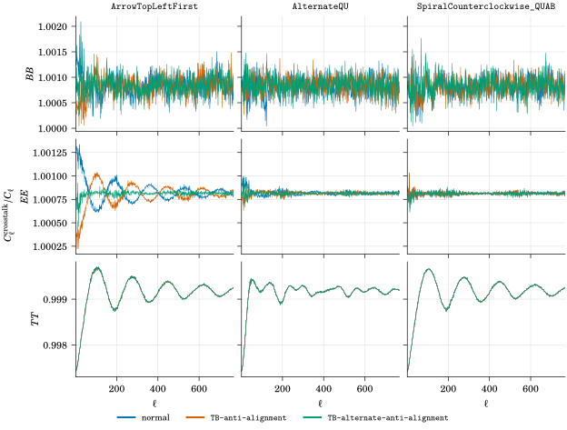
From fig. 36.8, one can observe,
in polarizations,
the \(B\)-mode power-spectra are noisier compared to the \(E\)-mode, but they follow a similar trend.
For walking order,
SpiralCounterclockwise_QUAB>AlternateQU>ArrowTopLeftFirst. It is basically determined by the amount of \(Q\)-\(U\) pixel crossing when walking the wafer.for \(TB\)-alignment,
TB-anti-alignmentis as bad as normal-ordering, andTB-alternate-anti-alignment-ordering is the best. As \(\sum_i \cos (2 \alpha_i) \approx 0\).
in \(TT\),
AlternateQUis better. As systematics are injected at different angular scales, so the Legendre polynomial term partially cancelled between different contributions. In fact, if we walk the wafer randomly, this effect would be maximized.
36.4 Conclusions
The \(QU\)-ordering optimization effectively removes crosstalk systematic bias in the resultant \(E\)-mode and \(B\)-mode power-spectra.
One reason that the SpiralCounterclockwise_QUAB family is so effective is that we can consider the ordering in a SQUID (below we use SpiralCounterclockwise_QUAB_TB-alternate-anti-alignment-wire_TB as an explicit example),
\[1QAT \rightarrow 1QAB \rightarrow 2UAB \rightarrow 2UAT \rightarrow 3QBT \rightarrow 3QBB \rightarrow 4UBB \rightarrow 4UBT \dots\]
Note that not only the nearest neighbor (in SQUID) is a nearest neighbor (in focal plane) crossing between \(Q\) & \(U\) pixels (such as \(1QAB\)-\(2UAB\)), but it is true for the next nearest neighbor too (such as \(1QAT\)–\(2UAB\)). So effectively this has mitigated the leading 2 orders of crosstalk in the matrices.
It is also superior in terms of physically wiring the wafer. For example, ArrowTopLeftFirst_TB-alternate-anti-alignment-wire_TB also has small bias due to \(\sum_i \cos (2 \alpha_i) \approx 0\), but it is considerably harder to wire because it requires a lot of crossing. Not to mention the other case AlternateQU_TB-alternate-anti-alignment-wire_TB which needs to go back and forth.
Instead, SpiralCounterclockwise_QUAB designs the wafer starting from how one wants to wire/walk them on the focal plane first, once that is done, \(Q\)/\(U\)-ness of the detectors is assigned accordingly. As the \(T\)/\(B\)-ordering does not matter in this design, one is free to choose the \(TB\)-ordering due to physical limitation (minimize crossing.)
We should emphasize that this mitigation technique depends on the presence of CRHWP, as its design is based on Corollary 2, which is derived from eq. (34.10), a consequence of an analytic model with a set of assumptions listed in Assumption 1. How well it generalizes to other CMB experiments remains to be explored. It is likely that any CMB experiments with CRHWP with a fairly large sky coverage and isotropic scanning strategy (which are typical design requirements) such as the SAT in SO can take advantage of this, because they fulfill Assumption 1 approximately.
If this mitigation technique is applied, the crosstalk requirements may, for example, be relaxed (which may allow a larger multiplexing factor and in turn lower the payload & cost) by using this mitigation method, but the \(BB\) systematics have to be studied more in detail at large crosstalk limit.
Note that a popular technique to mitigate crosstalk systematics is to perform matrix inversion to remove the crosstalk in the TOD. This requires an accurate measurement of the crosstalk matrix, and the systematic uncertainties will be dominated by how accurate the crosstalk matrix can be measured. The proposed technique here can be used together with the matrix inversion technique, such that any residual crosstalk in the TOD can be mitigated by this wafer ordering technique.
There remains more crosstalk systematics to be explored, such as time-dependent crosstalk, and cross-frequency crosstalk.
Lastly, another possible exploration of the analytical structure seen here is to perform likelihood analysis using the power-spectra with the \(P_\ell(\cos θ)\), \(d^\ell_{22}(θ)\) as templates with \(θ\) at some of the characteristic angular scales of the focal plane on the sky. This gives an advantage to remove residual crosstalk systematics, but reduces the statistical power of the experiment.
Footnotes
“Statistical Scatter in LC Resonators and LiteBIRD Crosstalk Simulations”.↩︎
Note, however, that this maximizes the \(E \rightarrow B\) leakage at 2nd order in \(x\). In practice, which rule is more advantageous depends on the separation of scales comparing higher-order crosstalk effects to the \(E\) to \(B\) hierarchy.↩︎
Assuming 1st order crosstalk is roughly constant.↩︎
Montgomery et al., “Performance and Characterization of the SPT-3G Digital Frequency Multiplexed Readout System Using an Improved Noise and Crosstalk Model”.↩︎