26 Timestream of Data (TOD)
POLARBEAR, Time-ordered data, Filtering, Beam, Calibration, Convolution, Half-wave plate
26 Timestream of Data (TOD)
As we have some general ideas about the pipelines from previous sections, let us go back and revisit some of the details involved. We should note that the low-\(\ell\) B-mode large-patch analysis is published already. All large-patch analyses share similar pipelines. The earlier a task is in the pipeline, the more it is shared among them. So here we are not repeating all the details but will refer to The POLARBEAR Collaboration et al.1 whenever possible.
We will start from the Timestream of Data (TOD). As we mentioned in sec. 9.3, when observing the CMB, which is inherently a 2D object, we instead scan the sky and obtain a TOD first2.
To expand upon eq. (10.1) to show all complications that arise in real-world observations,
\[\begin{align} m^{\prime}_{p} & = \mathcal{B} \mathopen{} \left \{ m_{p} \right \} \mathclose{} \label{eq:beamConvolution} \tag{26.1}\\ d \mathopen{} \left ( t \right ) \mathclose{} & = P_{t p} \left( m^{\prime I}_{p} + \eta \left( m^{\prime Q}_{p} \cos \mathopen{} \left ( 2 \psi_{t} \right ) \mathclose{} + m^{\prime U}_{p} \sin \mathopen{} \left ( 2 \psi_{t} \right ) \mathclose{} \right) \right) + N_{t} \label{eq:TODObservation} \tag{26.2}\\ d^{\prime} \mathopen{} \left ( t \right ) \mathclose{} & = \mathcal{D} \mathopen{} \left \{ d \mathopen{} \left ( t \right ) \mathclose{} \right \} \mathclose{} \approx \left( 1 + g d \mathopen{} \left ( t \right ) \mathclose{} \right) d \mathopen{} \left ( t - \tau d \mathopen{} \left ( t \right ) \mathclose{} \right ) \mathclose{} \label{eq:TODconvolution} \tag{26.3}\end{align}\]
Here, \(m_p\) represents the physical CMB map on the sky. And eventually \(d'(t)\) is the TOD recorded as raw data.
Eq. (26.1) represents the map that the telescope sees. This normally means it is a beam-convolved map, assuming the beam is symmetric for simplicity.
Eq. (26.2) represents how the telescope scans the sky and obtains a TOD. Note that the HWP angle \(\psi\) and the pointing \(P\) are involved, where both together constitute the scanning strategy which determines the observed signal. \(η\) represents the polarization efficiency of the detectors. And \(N\) is the noise of the detectors.
Lastly, eq. (26.3) represents a non-linear effect from the detectors which makes the observed TOD a convolved version of the actual TOD. The approximation is characterized in Takakura et al.3 eq. 2.9.
In fact, these describe the TOD observed per detector, so all parameters involved can depend on the individual detector.
While a scanning strategy determines \(P\) and \(\psi\), the observing pointing \(P\) and HWP angle \(\psi\) are recorded. For the pointing, as outlined in The POLARBEAR Collaboration et al.4 a \(5\)-parameter pointing model is used to reconstruct the pointing to reduce error from the actual pointing. In large-patch analysis, we followed a similar procedure to construct the pointing model using point sources.5
Eq. (26.1) means that we need to characterize the beam as well. The beam window function6 is measured using dedicated observations of Jupiter,7 and an effective beam is used across all detectors although they differ slightly across wafers. This is good enough as the differences between the beams are much less than the statistical error-bar at this noise level.
Then, we need to characterize the detectors including the polarization efficiency and the effect of detector non-linearity. The methodology of the latter is studied in Takakura et al.8 Detector time constants are measured by using a thermal source on the telescope, and polarization efficiency together with their polarization angles are calibrated using Tau A observation, as indicated in The POLARBEAR Collaboration et al.9
After all these calibrations, the TOD is deconvolved10 as an inversion of eq. (26.3), the mapmaker is effectively inverting eq. (26.2), and at a later stage the power-spectra are de-biased by the beam profile to invert the effect of eq. (26.1).
26.1 Time domain filtering
One key difference between the low-\(\ell\) and high-\(\ell\) pipelines is illustrated below.
As the naïve mapmaker is used in our analysis, filtering the TOD is one of the techniques we can count on as we are not performing un-biased mapmaking. One of the benefits of splitting the large-patch analysis into low-\(\ell\) and high-\(\ell\) pipelines is that we can use different amounts of filtering to suppress different levels of unwanted systematics. In high-\(\ell\), we can afford heavier filtering from the low-frequency end, as we do not need the low-\(\ell\) signals.
TOD filtering is an optimization problem. If too little, systematics are too large and null-tests will fail. If too much, we are eating into the signal and hurting the sensitivity.
One such example is the common-mode filter. Common mode means the mode common to all detectors. And it is estimated as the sample mean of those detectors at time \(t\). It can be understood in terms of Principal Component Analysis (PCA) that the common mode approximately corresponds to the principal component among the detectors. The subtraction of the common mode helps reduce the amount of \(1/f\) noise.
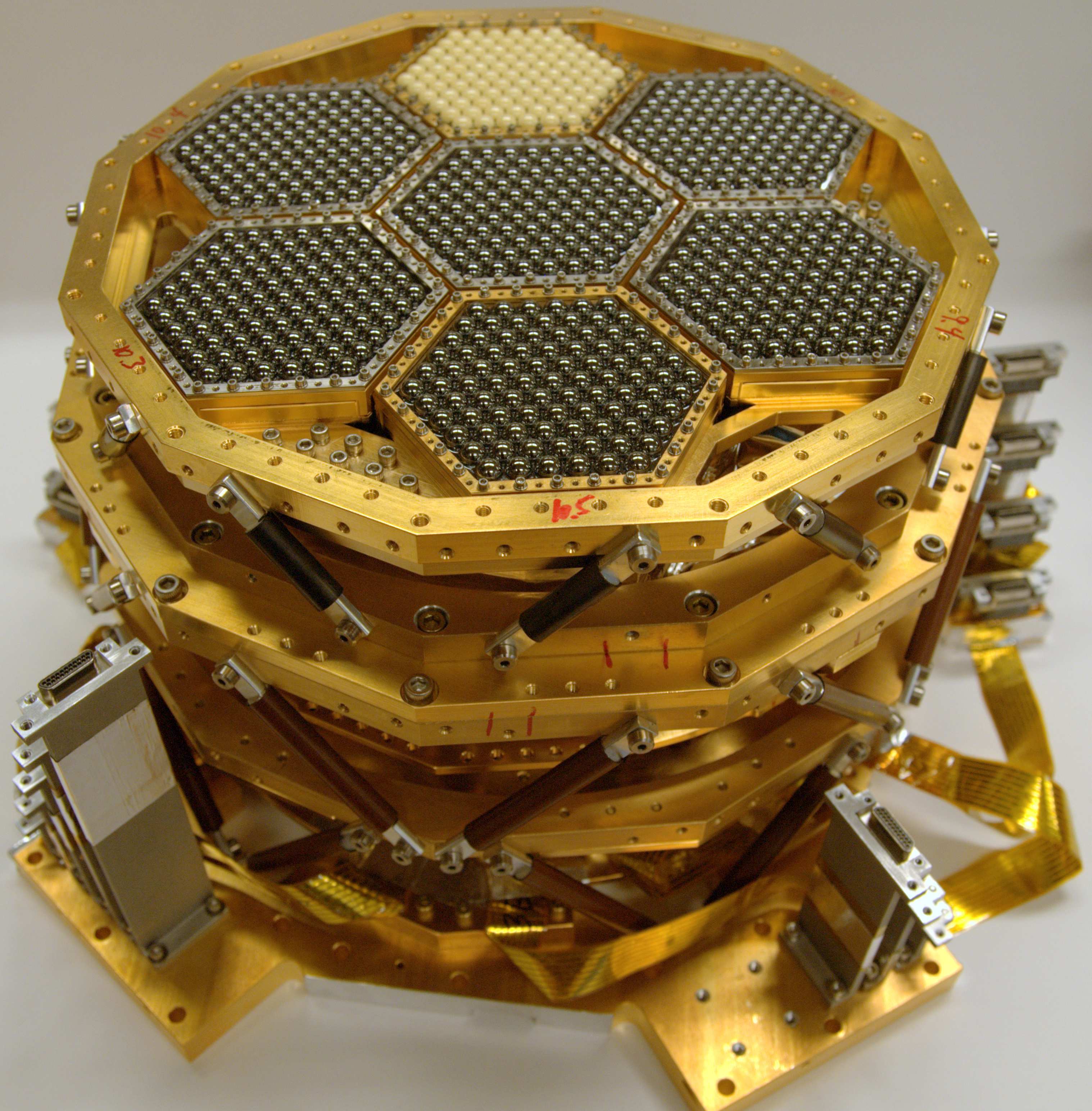
Note that common mode is constructed among a set of detectors. In low-\(\ell\), a single common mode is constructed over all detectors on the focal plane. As seen in fig. 26.1, a single wafer corresponds to a smaller angular scale on the sky, compared to the full focal plane12. Hence, the high-\(\ell\) pipeline can afford more aggressive filtering by constructing a common mode per wafer.
Similarly, we have polynomial filtering per sub-scan13 of the telescope. An \(n\)-th order polynomial is fitted in the TOD within each sub-scan and is subtracted from the TOD. This attempts to remove the long time scale fluctuation from the \(1/f\) noise, but also inevitably removes some of our large angular scale signal. Again, the high-\(\ell\) pipeline can afford a larger degree polynomial without eating too much into our science range here. In this specific research, a \(9\)-degree polynomial is fitted and subtracted from the TOD for all 3 components \(I, Q, U\).
Footnotes
“A Measurement of the Degree-Scale CMB B-Mode Angular Power Spectrum with POLARBEAR”.↩︎
“Performance of a Continuously Rotating Half-Wave Plate on the POLARBEAR Telescope”.↩︎
“A Measurement of the Cosmic Microwave Background B-Mode Polarization Power Spectrum at Sub-Degree Scales with POLARBEAR”.↩︎
The POLARBEAR Collaboration et al., “A Measurement of the Degree-Scale CMB B-Mode Angular Power Spectrum with POLARBEAR”.↩︎
This inherently assumes the beam is symmetric.↩︎
The POLARBEAR Collaboration et al., “A Measurement of the Degree-Scale CMB B-Mode Angular Power Spectrum with POLARBEAR”.↩︎
“Performance of a Continuously Rotating Half-Wave Plate on the POLARBEAR Telescope”.↩︎
“A Measurement of the Degree-Scale CMB B-Mode Angular Power Spectrum with POLARBEAR”.↩︎
This only applies to the real data but not the simulations as we do not simulate the detector non-linearity effects.↩︎
A total of \(7\) wafers are on the focal plane, where a smaller region on the focal plane corresponds to a smaller field of view on the sky.↩︎
A sub-scan corresponds to the duration where the telescope is constantly scanning in one direction. That is, each turn-around point marks the next sub-scan.↩︎