29 Running the Null-test suite
POLARBEAR, Null tests, Blind analysis, Systematics, Noise
29 Running the Null-test suite
29.1 Null-spectra
Let us take a look at an example null-spectra in fig. 29.1.
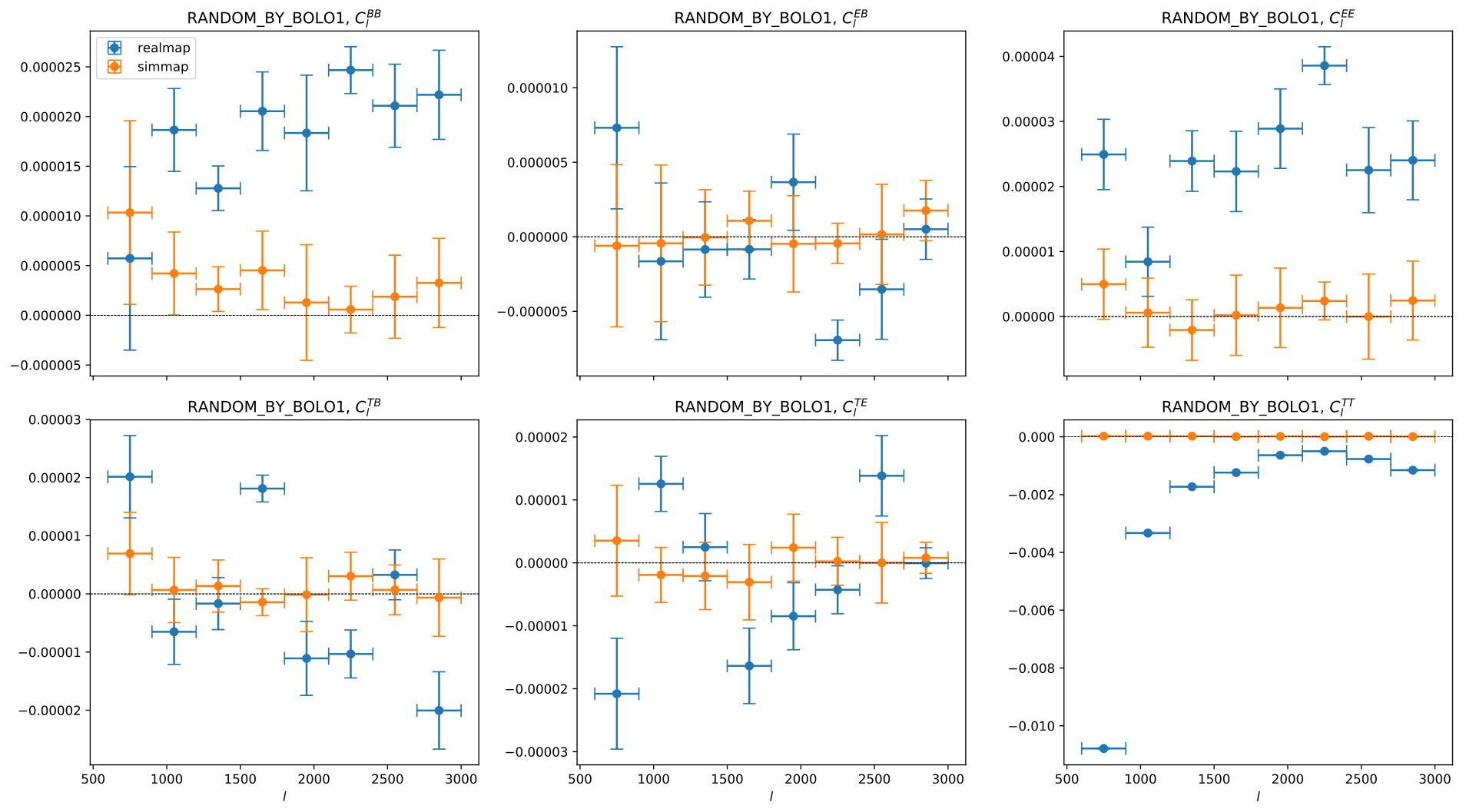
RANDOM_BY_BOLO1 null-spectra- The error-bars are estimated using \(n_\text{sim} = 8\) simulations that include fiducial signals and an uncorrelated white noise model with magnitude estimated from the TOD.
- The values of the simulations are averaged from all simulations to show you that this null-estimator is unbiased as we expect it to be consistent with \(0\) statistically.
- The values from the real data are the same null-estimator constructed using the observed TOD. Hence, this is where we might make “discovery” of unknown systematic effects.
(Normally, the vertical axis is in \(D_\ell\) scale, but here it is \(C_\ell B^2\ell\) for a reason that is going to be clear later.)
Just by looking at it, we can see that something is wrong with the \(BB, EE\) spectra. In fact, something is very wrong, as this null-split, RANDOM_BY_BOLO1, is randomly splitting the data into two halves according to which detectors it belongs to. And we do not normally expect a random-split to be failing.
Other null-test failures include
QU_PIXELLEAK_BY_BOLOAMP_2F_BY_BOLOAMP_4F_BY_BOLO
which are our discoveries in sec. 28.2.
29.2 Null-test failures
We named these failures as “local-by-bolo” splits, as they are all null-split by detectors that are separated locally on the focal plane.
For a long while, these null-test failures were not understood, and there was a long list of speculations as to why they are failing. And I checked each of these theories and falsified them:
- I-to-P leakage?
- Gain mismatch?
- \(1/f\) noise aliasing into \(4f\) frequency band contaminating the polarization signal?
- Requiring pairing of top and bottom detectors?
The actual problem and solution are discussed below.
The first hint is from fig. 29.1 when it was first plotted in \(C_\ell B^2\ell\) scale. Looking like white noise here is a huge hint. So we now know that this is a noise problem.
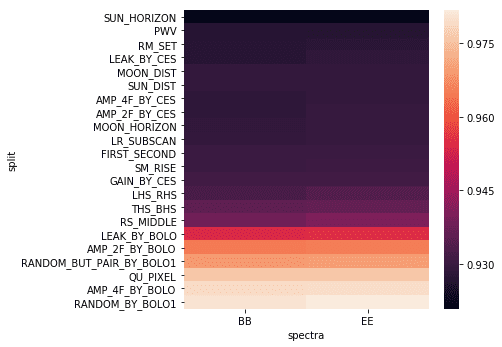
Further digging into the noise spectra, when the ratio between the real noise spectra and the simulated noise spectra is plotted in fig. 29.2, we have found the same set of null-splits that stand out from the others1.
Digging further, as pointed out by Goeckner-Wald2 in an internally circulated document, there is a bug in AnalysisBackend that added a term that should not exist in the calculation of the null-spectra, which normally would not be a problem as the expected value of this term is zero if the noise between the two splits is uncorrelated. But the very bug also gave us a hint of the origin of the problem—correlated detector noise. (Since different null-splits are splitting the same data in different halves, we know that the total noise level must be a constant and therefore this detector noise correlation is anti-correlating with some of the nearby detectors.)
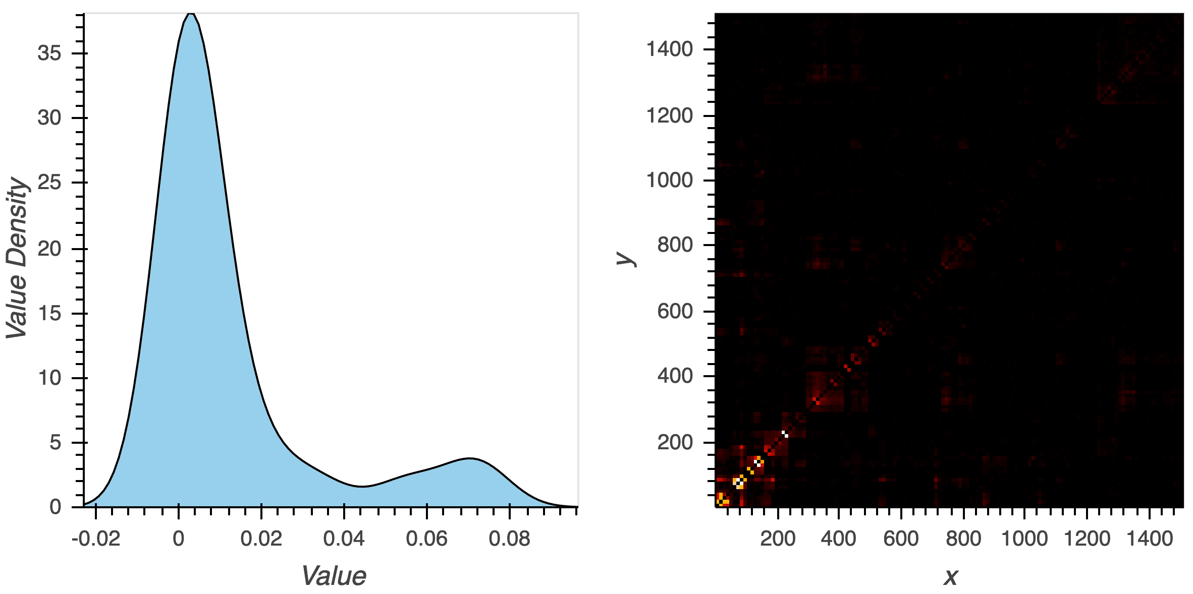
20141211_173206. R.H.S. shows a heatmap with the detectors reordered to reveal the clustering. On the L.H.S., \(\tilde{R_i} \equiv \max_j \left| r_{ij} \right|^2\) is first computed, and the Kernel Density Estimation (KDE) of \(\tilde{R_i}\) is calculated and shown here.The detector-detector correlations are calculated and a bad example CES is shown in fig. 29.3. These correlations are used to calculate a Kernel Density Estimation (K.D.E.) and there is a second peak. This gives us a data selection criterion, which is a classification problem, using the feature on the K.D.E. as the classification rule.
Our rule is then to find this 2nd peak per CES and cut away the data from the valley between them. This cuts away an additional amount of data volume at around \({5\,\%}\).
With all these fixes in-place, the null-spectra look like fig. 29.4.
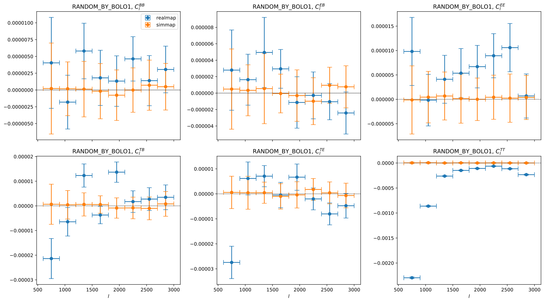
RANDOM_BY_BOLO1 null-spectraWe can see it is a huge improvement over fig. 29.1 for all of our science products \(EE, EB, BB\) power-spectra3.
29.3 When can we unblind?
As we are marching through the null-test iterations, the situation is improving.
The actual passing criteria are complicated, which includes other criteria such as Kolmogorov–Smirnov test mentioned in sec. 28.2.
But even focusing on the null-test suite alone, when are we going to end this endless pursuit of hidden systematics and be confident that we are good enough to unblind? In other words, what is the stopping criterion?
The first boring answer is to increase the number of simulations because they are not failing as dramatically and hence we need more accurate statistics to discern between fluke and discovery. But how much is enough?
This is a statistical problem. In short, we want to quantify how confident we are in passing the null-test before running the final run with hundreds of simulations.
The answer is confidence interval. But how do we estimate it? In Chinone,4 an erroneous argument is made following Clopper and Pearson,5 which uses an approximation that fails at the two extremes of the binomial, and is applied at one of the extremes \(p=0\).6
But we do not even have to fix that formula, instead, we can apply the bootstrap method on the MC simulations from existing preliminary null-test result using a smaller number of MC simulations.
For example, in null-test v0.13.4, I have \(n_\text{sim} = 48\) simulations. Using the bootstrap method, I can resample the \(n_\text{sim}\) simulations and estimate the confidence interval \(P(\alpha_c \geq 0.05)\).
Applying this procedure, the weakest statistics in v0.13.4 is from \(EB\), where I have \(\alpha = {6.2\,\%}\) and \(P(\alpha_c \geq 0.05) = {81.4\,\%}\).
Since we require all \(EE, EB, BB\) to be passing, this is good enough and a sign that we are good to go.
Footnotes
Do not worry about the overall normalization as it would be fixed later. Also, the two random null-splits are added when searching for hints on why this problem exists.↩︎
Note that the white noise model instead of the sign-flip noise is used, so the \(TT\) null-power-spectra are still not good. This is fixed in the final analysis. See sec. 27.6.↩︎
“THE USE OF CONFIDENCE OR FIDUCIAL LIMITS ILLUSTRATED IN THE CASE OF THE BINOMIAL”.↩︎
See more from Agresti and Coull, “Approximate Is Better Than ‘Exact’ for Interval Estimation of Binomial Proportions”; Thulin, “The Cost of Using Exact Confidence Intervals for a Binomial Proportion”.↩︎