23 Sensitivity projection
POLARBEAR, Error bars and sensitivity, Power spectra, Spherical harmonics, Beam, Noise, Gravitational lensing
23 Sensitivity projection
As we have mentioned in chapter 19, in the 3rd–5th seasons, POLARBEAR observed a sky area of \({670{^\circ}^{2}}\). This dissertation focuses on the high-\(\ell\) \(B\)-mode science product from this observation. Let us start with a back-of-the-envelope calculation to see what result we should be expecting.
Since we have a \({3.5'}\) beam, We can estimate the maximum \(\ell\) that we can resolve by using the rule of thumb
\[Δθ \sim \frac{180^\circ}{\ell}.\tag{23.1}\]
This is because for the spherical harmonics used in decomposing the CMB1,
\[Y_{\ell }^{m}(\theta ,\varphi )={\sqrt {{\frac {(2\ell +1)}{4\pi }}{\frac {(\ell -m)!}{(\ell +m)!}}}}\,P_{\ell }^{m}(\cos {\theta })\,e^{im\varphi } .\]
Since \(|m| \leq \ell\), the smallest periodicity of the magnitude in the \(φ\)-direction is exactly \(\frac{180^\circ}{\ell}\).
So, from a resolution of a \({3.5'}\) beam, we expect
\[\ell_\text{max} = \frac{180^\circ}{{3.5'}} \sim 3000.\]
For the minimum \(\ell\) we can measure, that is subject to different criteria. First, our large-patch is roughly \({45^\circ}\) wide, so using a similar estimate seems to suggest we can measure down to \(\ell \sim 4\). But there are other factors that come into play. The most important one is the \(\ell_\text{knee}\), a characteristic \(\ell\) scale determined by the presence of low frequency noise. It turns out that \(\ell_\text{knee} = 90\), which is the topic of the low-\(\ell\) paper.2
As mentioned in sec. 21.5, the pipelines are split into two at \(\ell = 600\). This work focuses on the high-\(\ell\) range of \(600\)–\(3000\).
In this \(\ell\)-range, we are observing the lensing \(B\)-mode. This lensing \(B\)-mode is predicted by, as the name suggests, the lensing effect of the \(E\)-mode power-spectrum that becomes a \(B\)-mode pattern. It has first been observed by POLARBEAR in its first two seasons of data in the range of \(500 \leq \ell \leq 2100\).3 A natural question to ask is how the sensitivity of this project would compare to that.
To do this, we need to know how the sensitivity should scale with sky-area and map-depth.
23.1 Knox Formula
According to Hivon et al.4 eq. 16-17,
\[\Delta C_l \approx \sqrt{\frac{2}{\nu_l}} \left( C_l + \frac{N_l}{B_l^2} \right)\tag{23.2}\]
\[\nu_b \approx (2 l + 1) \Delta l f_\text{sky, eff.}\]
\[f_\text{sky, eff.} \equiv f_\text{sky} \frac{w_2^2}{w_4}\]
where it is understood that the \(l\)-bins are half open intervals: \(b = [l - \frac{\Delta l}{2}, l + \frac{\Delta l}{2})\).
Here, \(C_\ell\) is the power-spectrum, \(Δ C_\ell\) is its error-bar, \(ν\) is the d.o.f., \(B_\ell\) is the beam, \(N_\ell\) is the noise spectrum, \(f_\text{sky}\) is the fraction of the sky observed. \(f_\text{sky, eff.}\) is the effective \(f_\text{sky}\) adjusted by the 2nd and 4th moment (\(w_2\) and \(w_4\) respectively) of the mask used in calculating the power-spectra from the maps.
Note that this formula is exact given \(\ell\) if the underlying random variables (including the \(C_\ell\) term and the noise term) are all Gaussian and independent. \(ν = 2 \ell + 1\) per \(\ell\), and the factor of \(f_\text{sky}\) adjusts for the fraction of the number of modes lost in not measuring the full sky. Hence the validity of this formula depends on how well these assumptions hold in practice.
Understanding what it means, we can estimate \(ν\) better,5
\[\nu_b \equiv \sum_{l - \frac{\Delta l}{2}}^{l + \frac{\Delta l}{2} - 1} (2l + 1) f_\text{sky, eff.} = 2 l \Delta l f_\text{sky, eff.}.\]
That is, the one Hivon et al.6 used over-estimated the error-bar a little bit, which becomes relatively negligible when \(\ell\) is large.
Now, let us move on to see how we can project the sensitivity knowing only how the noise and \(f_\text{sky}\) scale. Assuming noise-limited,
\[\Delta C_b \sim N_b \sqrt{ \frac{ 2 }{ \nu_b } } \propto \frac{n^2}{\sqrt{f_\text{sky}}}.\tag{23.3}\]
Here we introduce the map-depth \(n\) which is the square-root of the noise spectrum, and also usually put in a different unit. Typically, the noise spectrum has a steradian implicitly in its unit7. But map-depth is usually put in the unit of \({\text{µ}\mathrm{K}\,'}\) so a conversion from \({\mathrm{sr}}\) to \({{'}^{2}}\) (square-arcminute) is needed.
Method 1: Scaling by the change of sky area only
Consider only the change in sky coverage, if we decrease the sky area by a factor of \(r\),
\[f_\text{sky} \rightarrow \frac{ f_\text{sky} }{r},\]
\[n \rightarrow \frac{n}{ \sqrt{r} },\]
\[Δ C_\ell \rightarrow \frac{Δ C_\ell}{\sqrt{r}},\]
where the scaling of \(n\) is deduced from the scaling of the standard error of the mean, assuming the total amount of observation stays constant.
That is, the signal-to-noise ratio is increased by \(\sqrt{r}\).
In the first two seasons, POLARBEAR observed a sky area of \({25{^\circ}^{2}} \rightarrow r = 25 / 670\). The signal-to-noise ratio is expected to decrease by \(0.19\).
Since The POLARBEAR Collaboration et al.8 reports a statistical error of \(0.26\) on \(A_L\), we expect it to be around \(1.3\) in this measurement.
But we can do slightly better. To account for the difference in the number of seasons (2 vs. 3), deducing from the standard error of the mean again, the signal-to-noise ratio will decrease by \(0.19 \times \sqrt{\frac{3}{2}} = 0.23\), leading to an error of \(A_L\) to be around \(1.1\).
All these should have been known before the beginning of the 3rd season of observation9. And since \(A_L\) simply is the ratio of what we observed comparing to what we expect, its fiducial value is \(1\), That is, we should have expected the sensitivity to be less than \(1σ\).
Before we move on, let us improve this calculation slightly by using the actual number of observation hours. The POLARBEAR Collaboration et al.10 reports \({2800\,\mathrm{h}}\) of observations, while we have \({2985\,\mathrm{h}}\). That is, it is much less data volume than we would expect from the increase from \(2\) to \(3\) seasons. One of the reasons is the eruption of a nearby volcano on October 30th, 2015,11 among other mechanical problems. This means the signal-to-noise ratio is decreased by a factor of \(0.19 \times \sqrt{\frac{2985}{2800}} = 0.20\) instead, resulting in an error of \(A_L\) to be around \(1.3\).
Method 2: Estimated using the actual map depth in map domain
The map depth \(n\) can be estimated in the map domain directly.
Naïvely, this can be estimated by the deepest part of the map. Internally, it is reported to be \({4.5\,\text{µ}\mathrm{K}\,'}\)12 from the first two seasons of data, and \({16\,\text{µ}\mathrm{K}\,'}\) for the later three seasons.
Using eq. (23.3), we would expect the error-bar to be \(2.4\) times more, resulting in \(Δ A_L = 0.63\).
But this number is highly deceptive for two reasons. First, the absolute gain was not known at the time. Taking into account the absolute gain in hindsight, the map depth is \({18.4\,\text{µ}\mathrm{K}\,'}\), resulting in \(Δ A_L = 0.84\).
The more serious problem is that the map depth is highly irregular as seen in fig. 23.1, while the first two seasons have very uniform maps.
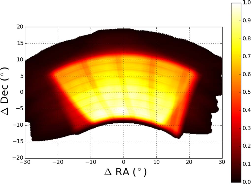
So a better metric would be to compare by their weighted average map depth. This is known internally to be \({5.5\,\text{µ}\mathrm{K}\,'}\) for the first two seasons and \({23.8\,\text{µ}\mathrm{K}\,'}\) for last three. This amounts to \(Δ A_L = 0.94\).
Method 3: Estimated using the actual map depth in power-spectra domain
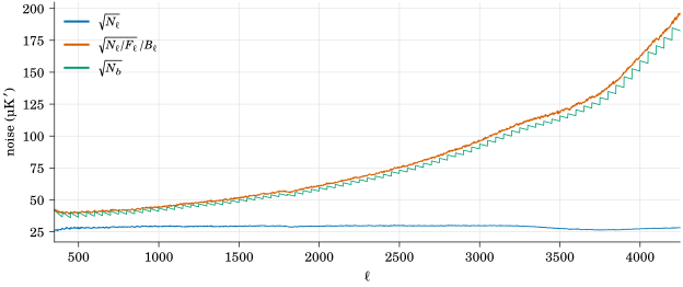
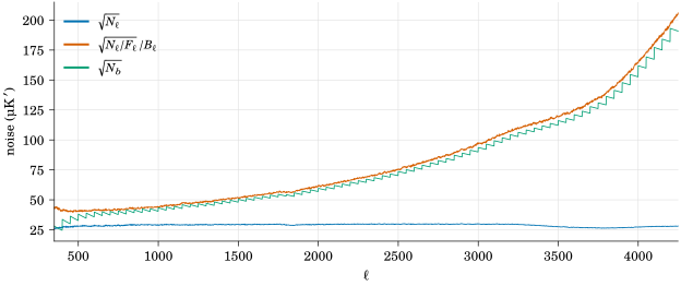
In fig. 23.2 and fig. 23.3, we plotted the noise spectrum. \(\sqrt{N_\ell}\) is the noise-spectrum, and the \(\sqrt{N_b}\) is the noise-spectrum after de-biasing using the MASTER algorithm,14 binned at a bin-width of 50. Since our science product is the de-biased power-spectra, \(\sqrt{N_b}\) should be the focus here.
Even if we are using the smallest value at \(\ell = 525\) which equals \({36.2\,\text{µ}\mathrm{K}\,'}\), comparing to an internally provided value from the first two seasons at \({6.3\,\text{µ}\mathrm{K}\,'}\), it would project to be \(Δ A_L = 1.7\).
Lesson learnt
To summarize, we should have projected the sensitivity to be \(Δ A_L = 1.1\) before the observation even started, and \(Δ A_L = 1.7\) in the beginning of the analysis.
But, all these were unknown to anyone in the collaboration at the time, including the very author who spent a few years in analysis. Hence, this is perhaps the most important but simple physics one should understand and calculate. Sometimes we got buried in details and got lost in the big picture.
However, all is not lost. As we shall soon see, this experiment shows that we can measure the polarization of the CMB in a wide range of \(50 \leq \ell \leq 3000\)15 using a single medium aperture telescope.
Footnotes
See Spherical harmonics for details.↩︎
The POLARBEAR Collaboration et al., “A Measurement of the Degree-Scale CMB B-Mode Angular Power Spectrum with POLARBEAR”.↩︎
The POLARBEAR Collaboration et al., “A Measurement of the Cosmic Microwave Background B-Mode Polarization Power Spectrum at Subdegree Scales from Two Years of POLARBEAR Data”.↩︎
“MASTER of the Cosmic Microwave Background Anisotropy Power Spectrum”.↩︎
Hamilton et al., “Sensitivity of a Bolometric Interferometer to the Cosmic Microwave Backgroud Power Spectrum”, eq. 20.↩︎
“MASTER of the Cosmic Microwave Background Anisotropy Power Spectrum”.↩︎
That is, the unit is simply \({{\text{µ}\mathrm{K}}^{2}}\) with the steradian not written explicitly.↩︎
“A Measurement of the Cosmic Microwave Background B-Mode Polarization Power Spectrum at Subdegree Scales from Two Years of POLARBEAR Data”.↩︎
While the slight difference in the use of \(\ell\)-range is not accounted for so far, it turns out to be negligible.↩︎
“A Measurement of the Cosmic Microwave Background B-Mode Polarization Power Spectrum at Subdegree Scales from Two Years of POLARBEAR Data”.↩︎
The POLARBEAR Collaboration et al., “A Measurement of the Degree-Scale CMB B-Mode Angular Power Spectrum with POLARBEAR”.↩︎
Hereafter for the RA23 patch out of 3 different patches only. See The POLARBEAR Collaboration et al., “A Measurement of the Cosmic Microwave Background B-Mode Polarization Power Spectrum at Subdegree Scales from Two Years of POLARBEAR Data” for its definition.↩︎
“A Measurement of the Degree-Scale CMB B-Mode Angular Power Spectrum with POLARBEAR”.↩︎
Hivon et al., “MASTER of the Cosmic Microwave Background Anisotropy Power Spectrum”.↩︎
For \(50 \leq \ell \leq 600\), \(E\)-mode is only used for calibration.↩︎