9 Noise in CMB observations
Noise, Ground-based observation, Scanning strategy, Half-wave plate, Time-ordered data, Fourier analysis
9 Noise in CMB observations
Now let us switch gears to talk about the noise properties. This has important implications on how the CMB is observed, how CMB experiments are designed, and even how CMB data is analyzed.
9.1 Atmospheric noise
When we talk about observation frequencies, ground based CMB experiments have extra constraints here.
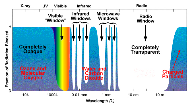
Take a look at fig. 9.1, we see that our choice of observation frequencies is limited by the atmospheric windows.
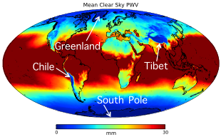
Not only that, from the precipitable water vapor (PWV) level across the world shown in fig. 9.2, we see that only some regions in the world favor CMB observations. It is because higher PWV, corresponding to red color in the figure, results in more absorption and therefore is less ideal for CMB experiments.
In fact, this is so important that all current ground based CMB experiments are in the low PWV regions shown as dark blue here2.
9.2 \(1/f\)-noise
Having mentioned the external factors involved in CMB experiments, we will briefly go through the actual instrument CMB experimentalists can design.
There is a lot of interesting physics involved in the design of these instruments. For example, it involves optical design of the telescope. And in detectors, there is Transition Edge Sensor (TES) bolometer which utilizes superconductivity to achieve photon-noise limited sensitivity. In detector readout, Superconducting Quantum Interference Devices (SQUIDs) are used to couple TESes together to achieve multiplexing, which enables us to pack a lot of detectors in a focal plane to beat down the noise.
But few of the characteristics of an instrument are as ubiquitous and have as profound implications as the following one we are going to mention: \(1/f\) noise.
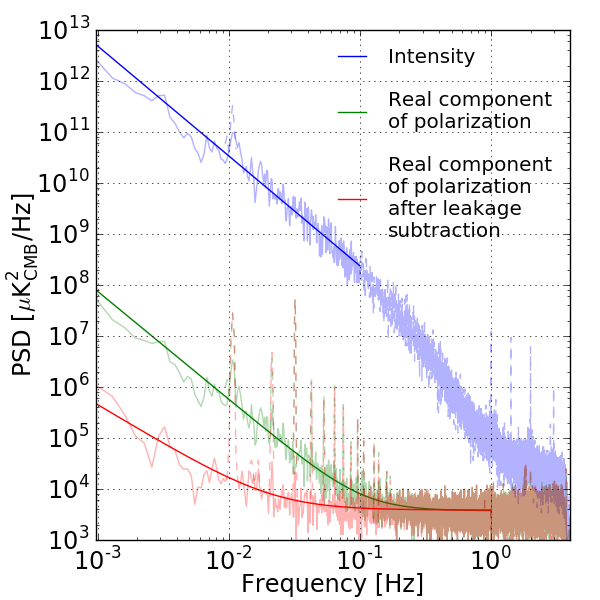
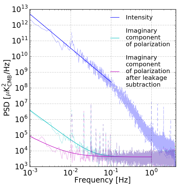
Figure 9.3: “PSDs of coadded timestreams for all focal plane detectors for the real part (left panel) and for the imaginary part (right panel). The blue line shows the intensity fluctuation and the green (cyan) and red (magenta) lines show the real (imaginary) part of the polarization signal before and after leakage subtraction, respectively. The spikes at the harmonics of \({0.01\,\mathrm{Hz}}\) are the scan synchronous signals.”3
From fig. 9.3, we can see an example spectrum of a detector TOD from POLARBEAR.
\[N \left[ 1 + \left( \frac{f_\text{knee}}{f} \right)^\alpha \right]\tag{9.1}\]
Eq. (9.1) describes the empirical form of noise like this. The first term is a white noise floor, and the second term is a straight line with slope \(\alpha\) on the log-log scale. This is the infamous \(1/f\) noise.
There are multiple sources that can lead to this empirical form, including atmosphere, electronics, temperature drifts, etc.
In this specific example, the atmosphere is the dominant contribution. But this is a fairly generic feature that appears in all our CMB measurements, and this characteristic affects how we design our experiments.
9.3 Scanning Strategy
The main implication here is that we cannot fixate on a point in space and measure the CMB, because in this static limit, where the frequency approaches \(0\), the noise level virtually diverges leading to a large uncertainty.
Instead, the rule of the game here is to modulate the signal, meaning that we make it change. That is, we change the signal such that it is no longer at zero frequency and away from the singularity.
That is why all CMB experiments have to design a scanning strategy to scan across the sky. This process is also called a differential measurement as effectively we are measuring the difference in the signal, the anisotropy of the CMB.
Because the CMB is not a scalar, having multiple components, cross-linking is also important. Cross-linking basically means that you revisit the same pixel with a different signal composition so that you can eliminate the degeneracy and solve for different signal components.
We are not going into the details of designing scanning strategy here, but we now focus on an interesting twist on scanning strategy below.
9.4 Modulation of the CMB signal via HWP
In measuring the CMB, \(1/f\) noise is less of a problem in measuring the Intensity, simply because the signal is big at low-\(\ell\), corresponding to low-frequency in the time-domain, which means we can afford larger noise-level there. But this is not the case for CMB polarization.
CMB polarization can be measured by pair-differencing—it takes 2 detectors at \({90^\circ}\) and takes the difference between them. But any non-ideality between the 2 is going to create Intensity to Polarization (I-to-P) leakage. For example, the 2 detectors might not be exactly at \({90^\circ}\), or might have different beam shape or band pass.
These make CMB polarization measurements more challenging.
One idea to solve these problems is to modulate the signal again, but to much higher frequencies utilizing polarization itself.
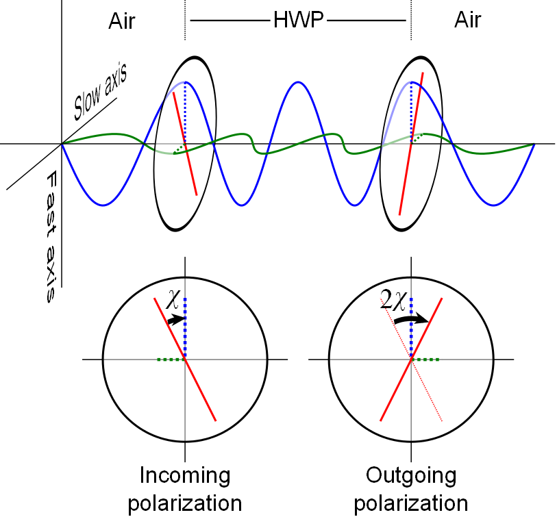
Fig. 9.4 is a Half-Wave Plate (HWP). What it does is that when light is transmitted through a HWP, the polarization angle will be reflected. We can then put the HWP in Continuous Rotation (CRHWP), and it will modulate any polarized components on the sky-side of the HWP by \(4\) times the frequency we rotate it. Note that this means the unpolarized components including atmospheric noise are left unmodulated. This separates the \(1/f\) infrared divergence region from the polarized signal at \(4f\).
In fig. 9.3, we see the effect of HWP demodulation, one of the techniques to reconstruct the original polarized components from the modulated signals which is detailed in chapter 22. We can see from the middle curve that \(1/f\) noise is hugely suppressed.
This kills \(2\) birds with one stone—it modulates the signals away from the \(1/f\) infrared divergence, and also enables a single detector to see both polarization modes, hence eliminating the need of pair-differencing and the associated systematics.
But there is still residual I-to-P leakage due to HWP systematics. It can include detector non-linearity, off-axis mirror, etc. It can be further suppressed in analysis using leakage subtraction as seen in the lowest curve.
In addition to these systematics, mitigation of \(1/f\) noise using HWP modulation is also limited by the presence of polarized noise components. HWP modulation can modulate such noise too, so that the signal is no longer separated from the infrared divergence. Takakura et al.4 provides one such example, where ice crystals in tropospheric ice clouds can create such polarized \(1/f\) noise components.
Footnotes
Barron et al., “Optimization Study for the Experimental Configuration of CMB-S4”.↩︎
This includes 4 regions—Chile, Antarctica, Greenland, and Tibet. The South Pole in Antarctica and the Atacama Desert in Chile are well-established sites for CMB observations for reasons outlined in Barron et al., “Optimization Study for the Experimental Configuration of CMB-S4”. 3 more sites—Ali in Tibet, Dome A in Antarctica, and Summit Camp in Greenland—are explored in Kuo, “Assessments of Ali, Dome A, and Summit Camp for Mm-Wave Observations Using MERRA-2 Reanalysis”. It concludes that, except for Greenland where a high level of liquid water clouds is detected, all remaining 4 sites are promising for CMB observations, where Ali in Tibet is the only one on the list which is “in the Northern Hemisphere that will complement well-established Southern sites”. Lastly, it should be noted that existing infrastructure in the South Pole and the Atacama Desert makes it favorable for future deployments.↩︎
Takakura et al., “Performance of a Continuously Rotating Half-Wave Plate on the POLARBEAR Telescope”.↩︎
“Measurements of Tropospheric Ice Clouds with a Ground-Based CMB Polarization Experiment, POLARBEAR”.↩︎