13 CMB power-spectra
Power spectra, Spherical harmonics, Gravitational lensing, Planck
13 CMB power-spectra
We have previously mentioned that we can obtain the power-spectra by performing spherical harmonics transformations and form \(TT\), \(TE\), \(EE\), \(BB\) spectra. But we have not mentioned why.
One reason is that maps are not unique. Our Universe is a random realization of fundamental physics and its parameters, and we as observers in the Universe are a random point-of-view. Changing either of these will change the map but not the power-spectra, as it is probing on the expectation values of these random fields.
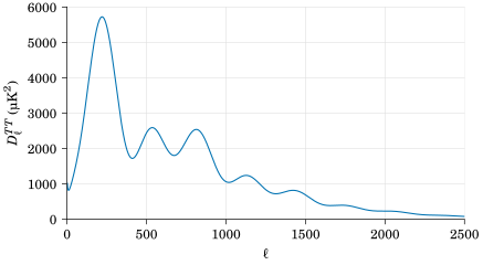
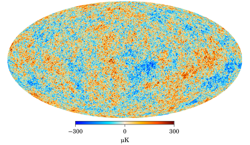
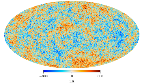
Here is a simple example that from the same power-spectrum in fig. 13.1, the one we measured here in the Universe is fig. 13.2, but fig. 13.3 is another random realization that yields the same spectrum!
Furthermore, theoretically we expect the primordial random fields to be nearly Gaussian, which is also not violated observationally. This means that the power-spectra as 2nd order statistics are sufficient statistics. That is, this is a lossless data compression, which further helps us to boost the signal-to-noise ratio.
This means that we can perform further systematic mitigation, such as unresolved point sources, gravitational lensing of the CMB by the foreground, or we can construct templates for systematic effects that are not mitigated in earlier steps.
13.1 Beyond 2-pt
Although we said that 2-pt statistics are sufficient statistics for the primordial CMB, the CMB we observed has non-linear, hence non-Gaussian distortion, for example by the gravitational lensing from the foreground. While this distorts all power-spectra, this affects B-mode the most as we have seen earlier.
In fact, the lensing potential can be constructed to describe the gravitational lensing effects, which can then be used together with the \(E\)-mode to produce a lensing \(B\)-mode template, which is what we have seen in fig. 5.3.