14 Simulations of CMB experiments
Simulations, Systematics, Error bars and sensitivity
14 Simulations of CMB experiments
Now that we have gone through all the major components needed for CMB data analysis, we can now look at the big picture of a general analysis pipeline in Fig. 14.1.
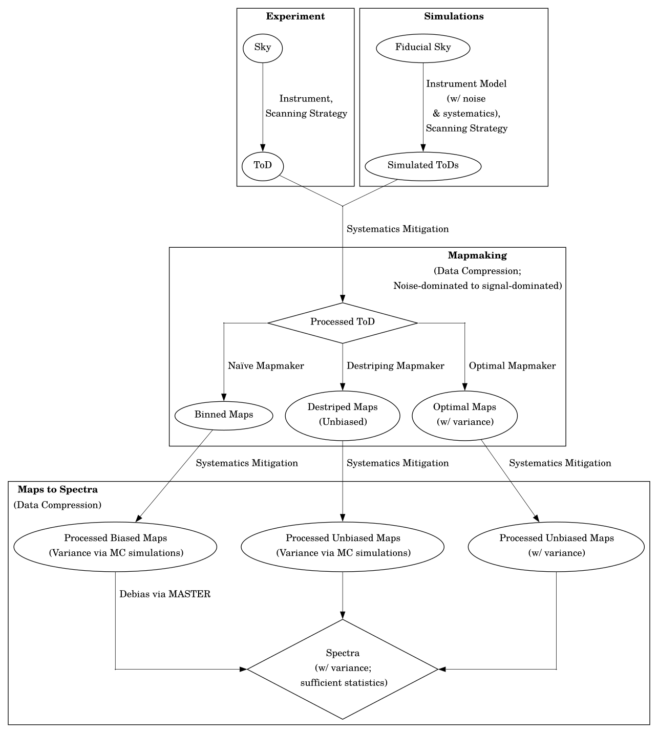
The only missing piece so far is the ability to simulate everything we said with an instrument model that captures the important characteristics such as scanning strategy, noise, systematic effects, etc.
There are many reasons we would need this. But the fundamental reason in our formulation here that we need simulation is that our mapmakers do not produce the covariance information due to computational constraints.
Therefore, we need to perform Monte Carlo (MC) simulations. We inject random noise with physical characteristics and use Monte Carlo method to estimate the statistical error in our final power-spectra. The typical number would be \(O(100-1000)\), which means that computationally we are trading off a higher time complexity to a lower one with a larger pre-factor.
Once we have this facility in place, we can use this to perform pipeline validation, often early in the process of designing an experiment, to demonstrate the correctness of the pipeline, and the capability of handling the observed dataset.
Also, we can use this to simulate systematic effects by injecting them into the data and measuring the outcome such as any biases and its associated error, and then devise systematic mitigation strategies and quantify their effectiveness.
Being able to simulate the statistical and systematic error, we can use this to perform forecasts which can inform experimental design.