25 Computational challenges
High-performance computing, Research software, Mapmaking, Null tests, Simulations, POLARBEAR
25 Computational challenges
25.1 Orientation
In the beginning, I was told to just run the whole pipeline with a smaller pixel at \({2'}\) and see what the null-test failures are. It was null-test v0.1.01.
However, I encountered multiple job failures because the nodes generated out-of-memory errors and/or exceeded the requested allocation time. It involved a lot of manual labor including fixing and rerunning whatever corrupted files when the jobs got killed.
Long story short, with 25 realizations2, it took me 1 month and the following amount of NERSC hours3:
- mapmaking: 33690 NERSC hours
- coadd: 55339 NERSC hours
- final-coadd: 86 NERSC hours
- mode-coupling matrices: ~70 NERSC hours
- pseudo-spectra: ~60,000 NERSC hours
I actually got the last one for free using the big-memory node at NERSC4. Had it been charged, it would have been a total of ~150,000 NERSC hours.
And if you are laughing right now, you understand that mapmaking is supposed to be the only expensive part. But here, co-adding is more expensive than mapmaking (where it is only doing weighted-sum), and pseudo-spectra pipeline is more expensive than co-add.
To put that time cost into perspective, I ran approximately 31 different null-test versions5 that involve at least the post-mapmaking pipelines.
Not only that, near the end of the analysis where we are closer to passing the null-tests, we increased our total number of realizations from 25 to 97. And we used \(769\) realizations in the final run. Had I been using the original pipeline for this, I would have used ~5.2 million NERSC hrs and 31 months of turnaround time for this alone. So by the time of publishing this dissertation, I would have been nowhere near passing the null-tests, and would have exhausted my NERSC allocation per year a dozen times already.
25.2 Low lying fruit
Essentially embarrassing parallelism can only be \({100\,\%}\) effective if you can feed each processor a job and the load is perfectly balanced. It turns out both of these are far from true in our pipelines with our large-patch map size requirements.
For example, in the mapmaking pipeline, recall from eq. (21.1), \(m^{i} = \mathcal{M} \mathopen{} \left \{ d^{i} \right \} \mathclose{} , i = 1 , \dots , n_{\text{CES}}\), the default configuration is to run an MPI job with as many processes as the number of CESes where \(n_\text{CES} = 3391\). So each job is waiting for the longest running job to finish.
In the end, I wrapped the AnalysisBackend mapmaking command line interface with a Python function interface6 and call it from an MPI script. With naïve random scheduling and using fewer MPI processes, the load balancing issue is solved and the total NERSC hours needed is decreased by around a factor of \(5\).
Another example is the coadd-pipeline from eq. (21.2) & eq. (21.3), \(w^{I , X , n}_{p} = \sum_{i \in I} w^{i , X , n}_{p} , M^{I , X , n}_{p} = \sum_{i \in I} M^{i , X , n}_{p}\). It is very inefficient, requiring \({40\,Gi\mathrm{B}}\) of memory per process, and has a bad reading pattern7. By rewriting it from scratch, it has a more balanced read pattern, memory use is reduced to \({\sim 135\,Mi\mathrm{B}}\), and since the problem is IO bound, multithreading is used, resulting in negligible NERSC hours needed comparing to mapmaking. Notice also from the inherent parallelism involved8, \(I = 1, \ldots, 38\), \(n = 1A, 1B, \ldots, 21A, 21B\), with a total of \(1535\)9 embarrassingly parallel tasks.
The last remaining computational problems are the mode-coupling matrices10 and maps-to-pseudo-spectra pipelines11, which I call the “post-mapmaking pipeline” in short. While the former does not seem to be expensive, it is a blocking dependency of the next step, making it also a target to shave the turn-around time.
I have a few iterations in accelerating these pipelines. Earlier attempts are more Pythonic and trying to be backward compatible. But these “duct-tape” solutions do not work well as they rely on the big-memory node which is a bottleneck both in terms of scaling out the applications to more simulations and its availability12.
25.3 Accelerating the post-mapmaking pipeline
Post-mapmaking pipeline includes everything after obtaining the maps, including the calculation of mode-coupling matrices and calculating the pseudo-spectra from maps.
Both of these are examples where it cannot be written efficiently using pure Python code that heavily relies on vectorization13.
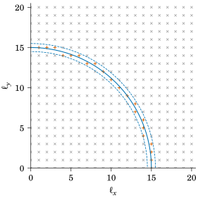
For example, in fig. 25.1, when calculating the pseudo-spectra from maps, the maps are first converted to frequency domain using Fast Fourier Transform (FFT), and since we are interested in \(\ell\), corresponding to the magnitude of the frequencies in the 2D-FFT, the values need to be binned down to individual \(\ell\).
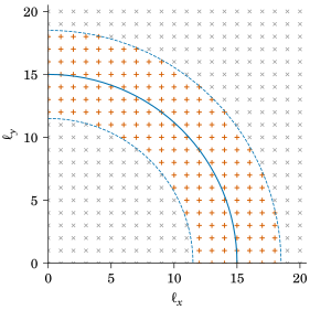
In fact, the original code relies on vectorization to first create a mask per \(\ell\), and calculate the averages by indexing arrays by this mask. Obviously it is very inefficient, but it also means that in order to get the job done in a reasonable amount of time, the averaging is done across an intermediate bin-width as shown in fig. 25.2.
Besides the computational problem, I found that the resultant binned null-spectra from this pipeline have different qualitative behavior depending on the bin-width used, for example, comparing fig. 29.1 & fig. 25.3. I suspect the use of this intermediate bin-width might be where the problem lies in its implementation in AnalysisBackend.
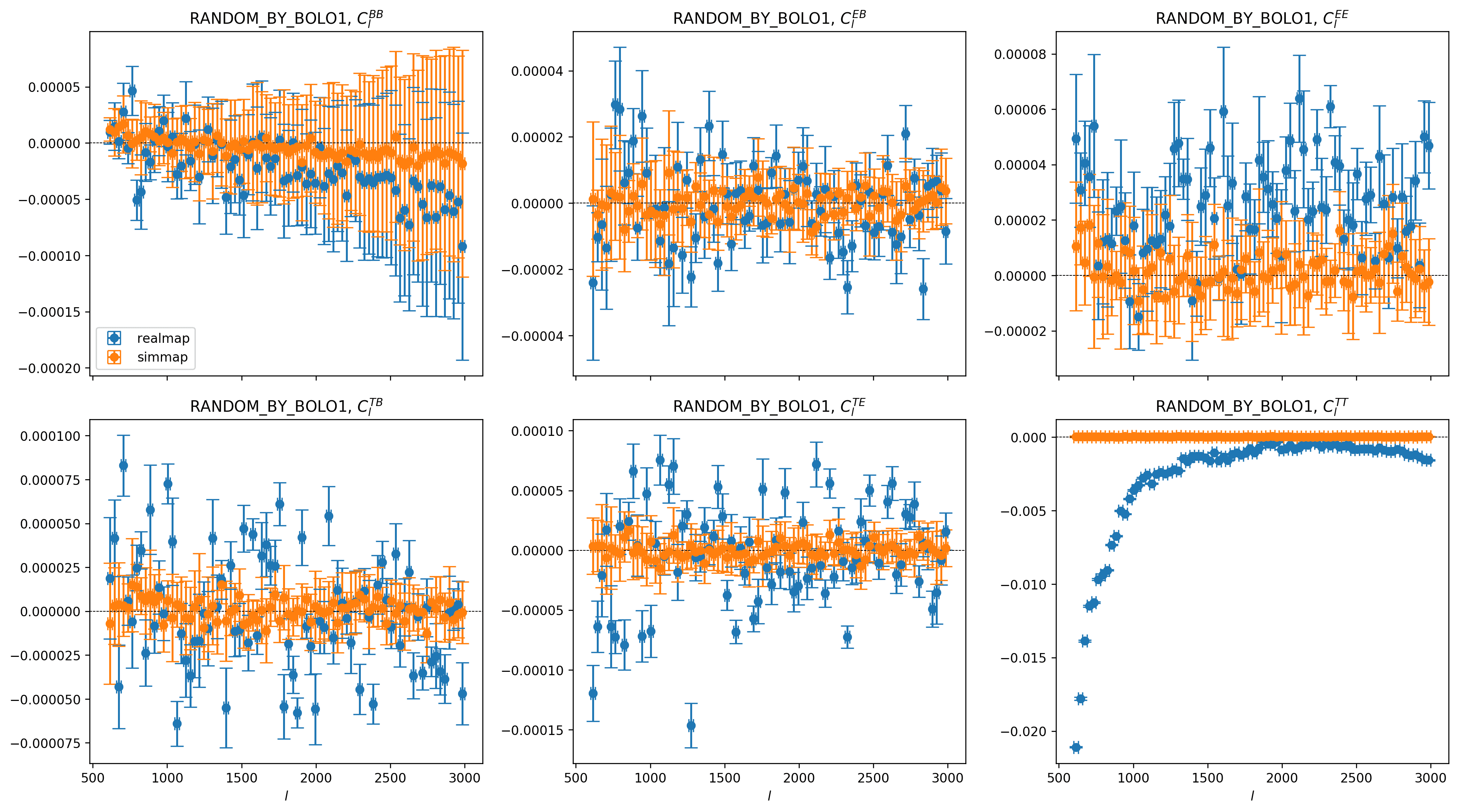
RANDOM_BY_BOLO1 null-spectra at finer bin-widthThe obvious first step is to proof-read the whole codebase to see where the problem lies and also how I might speed it up. Eventually, I found that it was easier to completely rewrite it.
In order for it to be performant, and as we have a policy of using Python only, I evaluated Cython and Numba, and in the end I chose Numba because it is easier to write Numba code that is guaranteed to release the GIL (nogil), is compiled to machine code (nopython), and is parallelized (parallel). Since Numba uses LLVM to just-in-time (JIT) compile the function, distribution is also effortless which is a bonus14.
This code is released as open source software on GitHub named TAIL, which stands for This Ain’t Interpreted Language.
Listing 25.1: Binning 2D spectra to 1D in Numba
# https://github.com/ickc/TAIL/blob/3b4e49d6d5a4/tail/pseudospectra.py
@jit(nopython=True, nogil=True, parallel=True)
def _bin_psd(pixel_size, l_max, psd):
    N = psd.shape[0]
    freq = fftfreq(N, pixel_size)
    n = l_max + 1
    psd_1d = np.zeros(n)
    hit = np.zeros(n, dtype=np.int64)
    pi_2 = np.pi * 2.
    for i in prange(N):
        freq_i = freq[i]
        for j in range(N):
            freq_j = freq[j]
            l = int(round(
                pi_2 * np.sqrt(
                    freq_i * freq_i +
                    freq_j * freq_j
                )
            ))
            idx = l if l < l_max else l_max
            hit[idx] += 1
            psd_1d[idx] += psd[i, j]
    psd_1d = psd_1d[:-1]
    hit = hit[:-1]
    ak_to_dl_scale = N * pixel_size
    ak_to_dl_scale *= 0.5 * ak_to_dl_scale / np.pi
    for i in range(l_max):
        hit_ = hit[i]
        psd_1d[i] = (
            (psd_1d[i] * ak_to_dl_scale / hit_) *
            (i * (i + 1))
        ) if hit_ > 0 else np.nan
    fill_nan(psd_1d, fill_boundary=False)
    return psd_1d
For example, one function from the pseudo-spectra pipeline is shown in lst. 25.1. Its style is quite C-like, and the prange there is similar to omp parallel for to explicitly parallelize the loop.
Listing 25.2: Python as Metaprogramming language of Numba
# https://github.com/ickc/TAIL/blob/3b4e49d6d5a4/tail/modecoupling.py#L128-L203
def _get_M_gen(Mtype, pure='hybrid'):
    if Mtype == 'TTTT':
        _J = _J_t
    else:
        _J_p = _get_J_p(Mtype, pure='hybrid')

        @jit(nopython=True, nogil=True)
        def _J(k1, k2, k3):
            return _J_t(k1, k2, k3) * \
                _J_p(k1, k2, k3)

    @jit(nopython=True, nogil=True)
    def simps(W, k1, k2):
        k3_min = np.abs(k1 - k2)
        k3_max = k1 + k2
        result = 0.
        for i, k3 in enumerate(
            range(k3_min + 1, k3_max)
        ):
            result += (2 - i % 2) * \
                _J(k1, k2, k3) * W[k3] * k3
        return result

    @jit(nopython=True, nogil=True, parallel=True)
    def _get_M(W, l_max, dl):
        bin_width = dl // 2
        n = l_max // dl
        M = np.empty((n, n))
        for i in prange(n):
            k1 = bin_width + dl * i
            for j in range(n):
                k2 = bin_width + dl * j
                M[i, j] = k2 * simps(W, k1, k2)
        return M

    return _get_M
An innovation in this code is the use of the Python language as a meta-programming language of the Numba language, for example as shown in lst. 25.2. The reason is that only a subset of the Python language can be compiled to machine code using Numba. So by writing higher order functions using the Python language which returns a Numba-jit-compiled function, we can achieve generality while being performant.
25.4 Results
In terms of turnaround time, note that each step of the pipeline is independent and each has a fundamentally different number of parallel jobs to do. There are \(n_\text{sim} \times n_\text{CES}\) mapmaking tasks, \(n_\text{sim} \times n_\text{map bundle} \times n_\text{null-split}\) coadd tasks, and \(n_\text{sim} \times n_\text{null-split}\) pseudo-spectra tasks. A key is to find the right MPI job size such that multiple pipelines can be put together into one single job script with one srun after another15.
By designing this carefully, the full null-test pipelines can be finished with 2 submissions to the NERSC queue via SLURM workload manager to minimize the queue time and hence the total turnaround time.
In the earlier phase when these are put together and we are still in the phase of solving null-test failures, the turnaround time is shortened from 1 month to typically a day, running exactly the same number of simulations.
As a testimony of the effectiveness of this short turnaround time, shortly after this is put in place, in 2 weeks I finished 6 iterations of null-test suites, leading to eventually the discovery and solution to our null-test failures.
In the final run with \(769\) realizations, instead of around \(5.2\) million NERSC hrs and 31 months of turnaround time, it only took me about \(440,000\) NERSC hrs and a few days to finish the first few hundred simulations (where I use the job array here to march through the queue more quickly.) This is a reduction of a factor of \(12\) in compute time, and a factor of a few hundreds in turnaround time.
Now that we have the computational challenge under control, we can turn our attention to what sort of problems we are facing when we are working towards unblinding.
Footnotes
I adopt semantic versioning in my null-test runs. See Changelog of null-tests performed in POLARBEAR large-patch analysis.↩︎
1 for the real data, 8 each for 3 kinds of simulations.↩︎
NERSC hour is a unit of computer time at the National Energy Research Scientific Computing Center (NERSC). It was calibrated to the computational power of 1 CPU core in an hour for an older NERSC system called Hopper. Exactly how much 1 NERSC hour is worth depends on calibration and it has been changed over time. During the time this analysis was done, on a Cori Haswell system where each node holds two Intel Xeon Processor E5-2698 v3 processors with \({128\,G\mathrm{B}}\) memory (See Cori - NERSC Documentation), 80 NERSC hours were charged when using 1 such node for an hour.↩︎
There are 2 such big-memory nodes at NERSC with \({750\,G\mathrm{B}}\). During the time of analysis, it was free to use but very congested.↩︎
around 30–40 depending on how you count. See Changelog of null-tests performed in POLARBEAR large-patch analysis.↩︎
It is a peculiarity in the design of AnalysisBackend that mapmaking can only be called from the command line using
argparse.↩︎It loads all combinations of \(X, n, p\) and \(i \in I\) in memory first.↩︎
I decided not to dispatch over \(X\) due to how the datasets are stored and the fact that there is enough parallelism.↩︎
It does not exactly equal \(38 \times 21 \times 2\) because some of the null-split maps would be empty.↩︎
I often need to wait from days to weeks to get into the queue.↩︎
The de facto standard in writing pure Python code in scientific computing is to use Numpy and the ecosystem built around it including Scipy. Numpy defines an array interface with syntactic sugars in Python with operations built around the concept of vectorization, and most of the operations are written as C modules, resulting in mostly efficient code. Limitations on its effectiveness originate from the Python data model, the generality of this array interface which is compiled AOT, and how effective vectorized programming can be on a particular algorithm.↩︎
In traditional ahead-of-time (AOT) compilation, the pre-compiled binaries should be compiled to optimize per architecture for each system. Since JIT compiler compiles at run-time which sees the CPU, it auto-optimizes for the target architecture without extra work, such as the Cori II KNL system which uses Intel Xeon Phi processors.↩︎
It is a limitation of the design in AnalysisBackend, which takes advantage of the embarrassingly parallel nature of our algorithms, to have each task read the inputs from disk and dump the outputs to disk. While this is an inefficient way of handling intermediate data by having IO on disk instead of holding it in memory, it does simplify the way to chain these independent pipelines together by using one
srunafter another when each pipeline has very different topology from each other.↩︎