28 Statistical methods
POLARBEAR, Hypothesis testing, Null tests, Likelihood and inference, Calibration, Gravitational lensing, Error bars and sensitivity, Simulations
28 Statistical methods
28.1 Absolute Gain Calibration
Keating, Shimon, and Yadav1 shows that we can use the CMB itself to perform absolute gain and angle calibration. Absolute gain refers to an overall factor multiplying the power-spectra, absolute angle refers to an overall angle rotating the linear polarization of the CMB. In a later section, we will show how they are estimated and corrected for in this analysis.
Cosmic variance limit
Let us first start by investigating a toy model where there is no noise. This is often coined as the cosmic variance limit, as it is an intrinsic uncertainty from the universe even if we can observe perfectly.
We have already seen the Knox formula eq. (23.2), in the limit of no noise,
\[\Delta C_\ell \approx \sqrt{\frac{2}{\nu_\ell}} C_\ell.\]
Defining absolute gain \(\alpha\)2 as
\[C_b^\text{obs.} = \alpha C_b^\text{Th.}\]
\[\alpha_b = \frac{C_b^\text{obs.}}{C_b^\text{Th.}}\]
\[\Delta \alpha_b \approx \sqrt{\frac{2}{\nu_b}}\]
Now, we assume a naïve OLS procedure assuming they are uncorrelated3 random variables as a function of \(b\), the corresponding standard error will then be
\[\begin{align*} \Delta &= \left( \sum_b \frac{1}{(\Delta \alpha_b)^2} \right)^{-\frac{1}{2}} \\ &= \left( \sum_b \frac{\nu_b}{2} \right)^{-\frac{1}{2}} \\ &= \left( \sum_b \frac{\sum_{l \in b} (2l + 1) f_\text{sky, eff.}}{2} \right)^{-\frac{1}{2}} \\ &= \left( \sum_{l = l_\text{min}}^{l_\text{max}} (2l + 1) \frac{f_\text{sky, eff.}}{2} \right)^{-\frac{1}{2}} \\ &= \left( \frac{(l_\text{max} + 1 - l_\text{min}) (l_\text{max} + 1 + l_\text{min})}{2} f_\text{sky, eff.} \right)^{-\frac{1}{2}} \\ \end{align*}\]
Note that this is independent of the actual binning \(b\) used.
Using our actual data, \(f_\text{sky, eff.} \approx 0.0159\).
With \(l_\text{min} = 600, l_\text{max} + 1 = 3000, \Delta \approx 0.00381\).
Method 1
Using \(C_l^{TT}\), the error of the absolute gain calibration \(\alpha\) is \(\Delta\).
Method 2
Using \(C_l^{EE}\), the \(\alpha\) estimated above is the product of the actual absolute gain times the polarization efficiency squared. That is,
\[\hat{\alpha} = \frac{\alpha^E}{\eta^2}\]
\[\left( \frac{\Delta \alpha}{\alpha} \right)^2 = \left( \frac{\Delta}{\alpha^E} \right)^2 + \left( 2 \frac{\Delta \eta}{\eta} \right)^2\]
Assuming \(\alpha \sim 1, \frac{\Delta}{\alpha^E} \sim \Delta \approx 0.00381\).
From internally circulated data, \(\frac{\Delta \eta}{\eta} \approx 0.0151\).
Method 3
Inverse variance weighted between method 1 & 2.
Since \(2 \frac{\Delta \eta}{\eta} \gg \frac{\Delta}{\alpha}\), the error bar obtained here is virtually identical to method 1.
Conclusion
In the cosmic variance limit, using the temperature data to estimate the absolute gain is much more accurate as the uncertainty in the polarization efficiency dominates the uncertainty in the case of polarization4.
This toy model illustrates why we would want to include the temperature power-spectrum for absolute gain calibration. With it, another bonus is that we can cross-check if the polarization efficiency is correct in the sense that the “absolute polarization efficiency” should be consistent with \(1\). Later we will see how this compares with the absolute gain inferred using the actual data.
28.2 POLARBEAR null-test framework in equations
In chapter 20, we already have an overview of the POLARBEAR null-test framework.
We see null-spectra are defined there. During the early phase of running null-tests, we can intuitively see what null-tests are failing where there are huge outliers. But we can do better to decide this objectively.
It involves constructing null-estimators from null-power-spectra. Exactly how these statistics are constructed is somewhat arbitrary. The POLARBEAR Collaboration et al.5 described the 5 different statistics used in the small-patch analysis over 3 different sky regions resulting in a total of 15 statistics. The definitions of the 5 statistics are somewhat vague, and the way the 15 statistics are combined is not specified.
There is also an internally circulated document Chinone6 documenting this null-test framework in more details.
Below we will mathematically define these quantities in this analysis.
Definition 1. Null-power-spectra.
Define random variable \(\chi(X, n, b) \equiv \frac{\hat{C}^{Xn, \text{null}}_b}{\hat{σ}^{Xn}_b}\) as a function of
\(X\): power-spectrum. This includes \(TT, TE, TB, EE, EB, BB\).
\(n\): null-split, such as AMP_4F_BY_BOLO, …
\(b\): an \(\ell\)-bin, such as \(600 \leq \ell < 700\).
Note that by construction, \(\chi\) is a standard score, assuming the theoretical expected value of \(0\), and estimated using the sample standard deviation via MC simulations. Asymptotically in \(n_\text{sim}\) and \(ν\), \(\chi \xrightarrow{d} N(0, 1)\).
Definition 2. Null-statistics.
Per spectrum, we collapse the null-power-spectra into the following 5 different ways,
\[Y_1(X) = \lvert \langle \chi(X, n, b) \rangle_{n, b} \rvert\]
\[Y_2(X) = \max_{n, b} \chi^2(X, n, b)\]
\[Y_3(X) = \max_{n} \sum_b \chi^2(X, n, b)\]
\[Y_4(X) = \max_{b} \sum_{n} \chi^2(X, n, b)\]
\[Y_5(X) = \sum_{n, b} \chi^2(X, n, b)\]
Consider sample space \(\Omega\).
\[Y_i: \Omega \rightarrow \mathbb{R}\]
\[Y_i: s \mapsto y_i\]
\[G_{Y_i}(y_i) \equiv P(Y_i > y_i)\]
Since \(G \equiv 1 - F\), \(G_{Y_i} \rightarrow U(0, 1)\)
Note that \(F\) is the cumulative distribution function (CDF) in statistics, while \(G\) is one minus that, often called probability-to-exceed (PTE).
In this analysis, the 5 statistics \(G_{Y_i}(y_i)\) are considered, by estimating the distribution of \(Y_i\) empirically through Monte Carlo simulation, and \(y_i\) from measured data. Additionally, 3 spectra are considered in the unblinding criteria: \(BB, EB, EE\). That is, there are a total of \(15\) p-values.
Theorem 1. Direct computation of null-statistics assuming \(\chi(X, n, b) \xrightarrow[i.i.d.]{d} N(0, 1)\).
\[\begin{align*} G_{Y_{1}} \mathopen{} \left ( y_{1} \right ) \mathclose{} & = \operatorname{erfc} \mathopen{} \left ( \sqrt{\frac{n_{\text{split}} n_{\text{b}}}{2}} \left| y_{1} \right| \right ) \mathclose{} \\ G_{Y_{2}} \mathopen{} \left ( y_{2} \right ) \mathclose{} & = \frac{n_{\text{split}} n_{\text{b}}}{2^{\frac{1}{2}} \Gamma \mathopen{} \left ( \frac{1}{2} \right ) \mathclose{}} \int_{y_{2}}^{\infty} \left( P \mathopen{} \left ( \frac{1}{2}, \frac{u}{2} \right ) \mathclose{} \right)^{n_{\text{split}} n_{\text{b}} - 1} \mathrm{e}^{- \frac{u}{2}} u^{\frac{1}{2} - 1} \,\mathrm{d} u \\ G_{Y_{3}} \mathopen{} \left ( y_{3} \right ) \mathclose{} & = \frac{n_{\text{split}}}{2^{\frac{n_{\text{b}}}{2}} \Gamma \mathopen{} \left ( \frac{n_{\text{b}}}{2} \right ) \mathclose{}} \int_{y_{3}}^{\infty} \left( P \mathopen{} \left ( \frac{n_{\text{b}}}{2}, \frac{u}{2} \right ) \mathclose{} \right)^{n_{\text{split}} - 1} \mathrm{e}^{- \frac{u}{2}} u^{\frac{n_{\text{b}}}{2} - 1} \,\mathrm{d} u \\ G_{Y_{4}} \mathopen{} \left ( y_{4} \right ) \mathclose{} & = \frac{n_{\text{b}}}{2^{\frac{n_{\text{split}}}{2}} \Gamma \mathopen{} \left ( \frac{n_{\text{split}}}{2} \right ) \mathclose{}} \int_{y_{4}}^{\infty} \left( P \mathopen{} \left ( \frac{n_{\text{split}}}{2}, \frac{u}{2} \right ) \mathclose{} \right)^{n_{\text{b}} - 1} \mathrm{e}^{- \frac{u}{2}} u^{\frac{n_{\text{split}}}{2} - 1} \,\mathrm{d} u \\ G_{Y_{5}} \mathopen{} \left ( y_{5} \right ) \mathclose{} & = Q \mathopen{} \left ( \frac{n_{\text{split}} n_{\text{b}}}{2}, \frac{y_{5}}{2} \right ) \mathclose{} \end{align*}\]
\(P\) and \(Q\) are the regularized lower incomplete gamma function and the regularized upper incomplete gamma function respectively.7 \(n_\text{split}\) is the total number of null-splits, \(n_\text{b}\) is the total number of \(b\)-bins.
It is trivial to prove these formulae when we realize \(\max\) is a special case of ordered statistics where the general formula is known. Proof is left as an exercise to the readers.
With these formulae, we do not need to estimate the PTE via MC simulations. Hence, it is much faster to evaluate and can act as an independent cross-check by comparing both approaches. We expect them to be similar, but note that the latter approach makes a qualitative assumption. Hence, the PTEs from MC simulations are the ones used in the unblinding criteria.
Note that all special functions are available in Scipy8, and the integral can be evaluated numerically. A Python implementation of these functions is available as p_1, …, p_5 in the stats module in TAIL.
| power-spectra | \(G_{Y_1}\) | \(G_{Y_2}\) | \(G_{Y_3}\) | \(G_{Y_4}\) | \(G_{Y_5}\) |
|---|---|---|---|---|---|
| BB | 82.8 % | 40.2 % | 52.1 % | 46.9 % | 14.5 % |
| EB | 79.7 % | 31.2 % | 35.9 % | 55.9 % | 7.6 % |
| EE | 36.5 % | 97.7 % | 90.4 % | 99.4 % | 83.4 % |
| TB | 8.6 % | 59.6 % | 98.8 % | 96.1 % | 89.1 % |
| TE | 17.0 % | 84.2 % | 59.2 % | 86.1 % | 85.9 % |
| TT | 17.2 % | 1.6 % | 9.0 % | 3.5 % | 6.6 % |
| power-spectra | \(G_{Y_1}\) | \(G_{Y_2}\) | \(G_{Y_3}\) | \(G_{Y_4}\) | \(G_{Y_5}\) |
|---|---|---|---|---|---|
| BB | 79.5 % | 43.9 % | 53.1 % | 40.4 % | 13.1 % |
| EB | 76.2 % | 32.8 % | 36.7 % | 53.1 % | 5.8 % |
| EE | 26.9 % | 97.4 % | 90.2 % | 99.0 % | 85.2 % |
| TB | 4.8 % | 61.6 % | 98.2 % | 96.3 % | 90.6 % |
| TE | 11.2 % | 86.1 % | 58.8 % | 83.8 % | 85.6 % |
| TT | 2.3 % | 0.0 % | 0.0 % | 0.1 % | 1.2 % |
As an example, here we show the comparison between the two estimates in tbl. 28.1 and tbl. 28.2 using null-test v1.0.0.
The general agreement between the two is a cross-check that they are behaving as we expected. The disagreements from the null-statistics generated using the \(TT\) power-spectrum is evidence that the assumption is not valid there. Fig. 28.4 further confirms the i.i.d. assumption is invalid. As explained in sec. 28.2, tbl. 28.1 is used in the unblinding criteria.
Kolmogorov–Smirnov test
From the real map, we obtained \(\chi^\text{real}(X, n, b)\). From n simulated maps, we obtained \(\chi^{\text{sim}, i}(X, n, b)\). A Kolmogorov–Smirnov test between \(\chi^\text{real}(X, n, b)\) and \(\chi^{\text{sim}, i}(X, n, b)\) is performed. This is often to ensure the simulation is statistically similar to the real observation such that the passing of the null-test would not be too optimistic9.
Correlations between null-splits
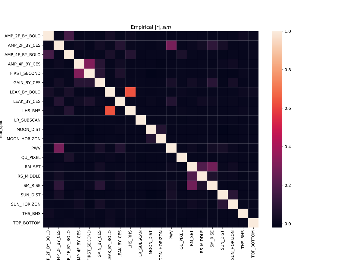
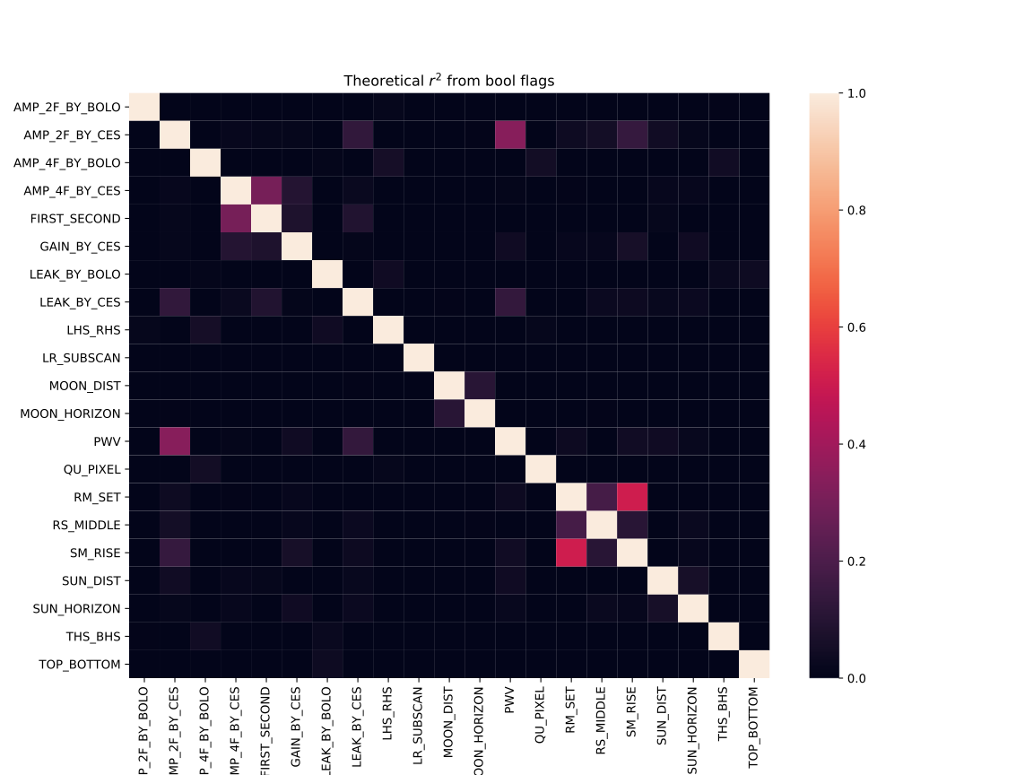
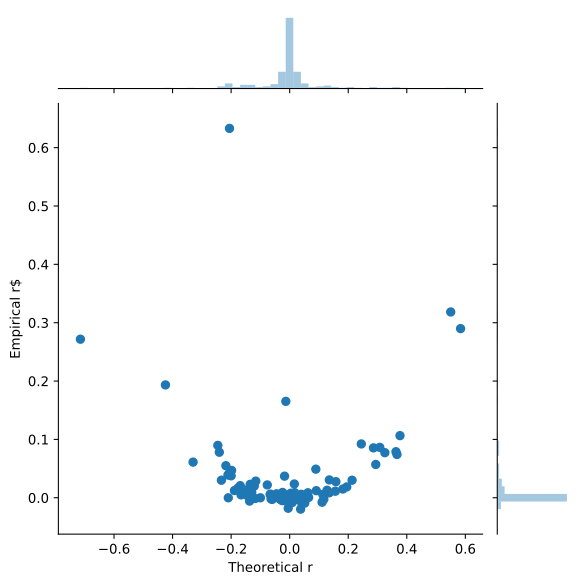
Fig. 28.1 tells us the empirical correlations between null-splits using their corresponding null-spectra. Fig. 28.2 shows the square of the correlation between the boolean flags of the null-split definition10. Under the ideal condition that the TOD has identical noise properties, we can predict that \(r_\text{empirical} \approx r_\text{boolean}^2\). Fig. 28.3 shows that this is also empirically true.
As you can see, since we are splitting the same dataset differently, they are correlated.
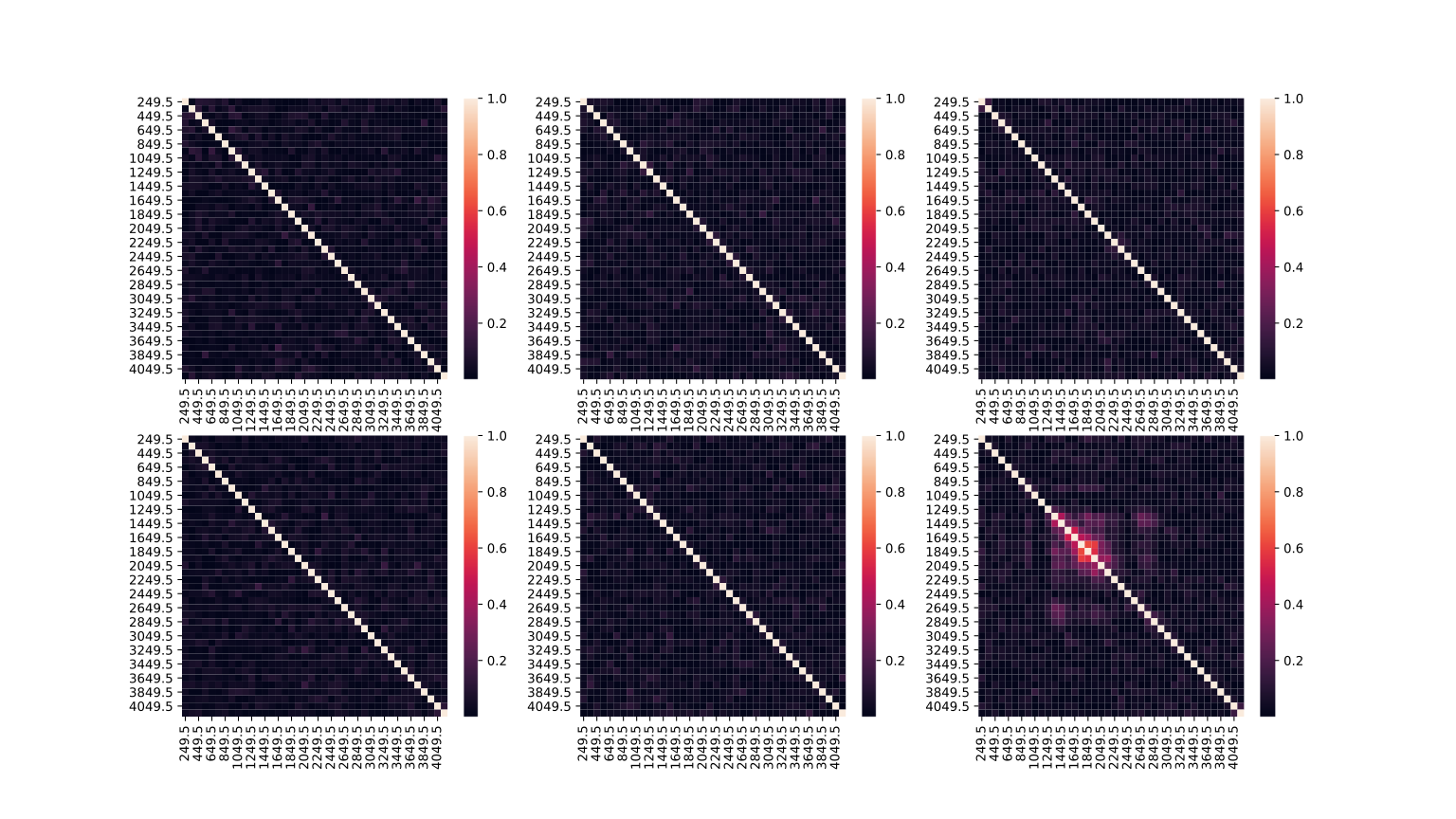
Similarly, from fig. 28.4 we see that the bin-bin correlations are negligible in all but the \(TT\) power-spectrum. Note that the HWP \(2f\) frequency corresponds to \(\ell = 1800\).
And if 2 null-splits are highly correlated, they are somewhat redundant with each other. Since we are performing a kind of sum over them in null-statistics, a natural question to ask is, given 2 of them have non-negligible correlations, should we choose only one of them? If we only choose one in the passing criteria, how can we be sure that is the correct choice, that is, the other one will equally pass the test?
Null-test selection and partial correlation
First, independence implies no correlations, but not vice versa.
As defined in definition 2, our null-statistics are complicated functions of the null random variable \(χ\). It is a misconception among some physicists that somehow the Pearson correlation coefficient is more physical, and if we find it to be small between 2 null-splits, their resultant \(5\) null-statistics will also be fairly independent.
Moreover, even if we find 2 null-splits to be highly correlated, are they still that much correlated after the correlation with other null-splits is taken into account?
A statistical way to quantify this is the partial correlation matrix, which can be written as
\[ρ_{χ_i, χ_j | χ_{k \neq i, j}, \ldots},\]
which is defined as the correlations between the residuals \(r_{χ_i | χ_{k \neq i, j}, \ldots}\) and \(r_{χ_j | χ_{k \neq i, j}, \ldots}\).
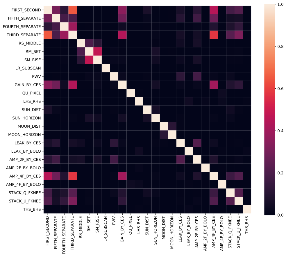
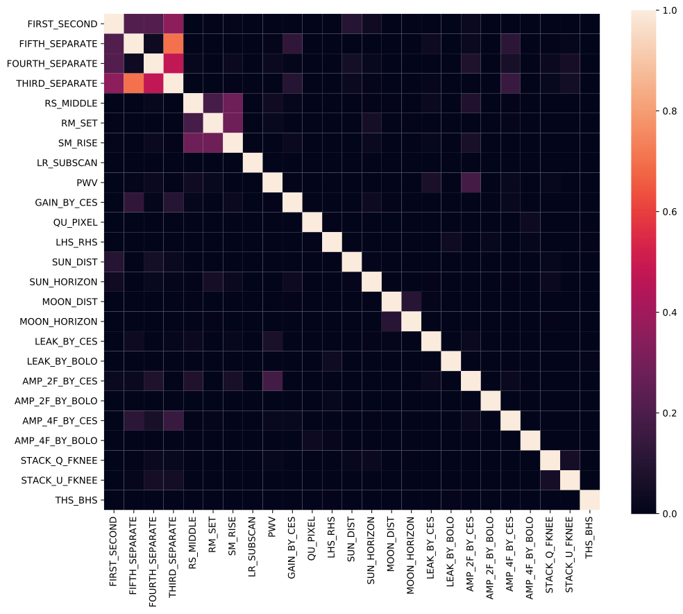
fig. 28.5; fig. 28.6 show the difference between the correlation matrices. The takeaway message here is that 2 null-splits can be apparently highly correlated, but much of the correlations can be explained by the rest of the null-splits. Hence, if one of them is excluded in the final null-test suite, it actually helps less than expected in removing dependencies.
In the end, the author suggests not to exclude null-splits in passing criteria based on some apparent correlations between them. Often, a null-split is defined by some physical observables with clearly defined meaning that should increase our confidence in the lack of systematics if the null-test suite passes. However, some can be excluded if there are strong reasons behind them. Here for example, we see that in earlier null-test v0.2.0 shown in fig. 28.5, there were more null-splits including THIRD_SEPARATE, FOURTH_SEPARATE, FIFTH_SEPARATE, which are defined as the 3rd season of data vs. the rest, and so on. Since FIRST_SECOND splits the data in the two halves chronologically, these 4 null-splits are quite redundant with each other. Since splitting the data in a half in data volume maximizes the sensitivity of the null-spectra, only FIRST_SECOND is kept in the final analysis.
Combined statistics—Family-wise Error Rate (FWER)
Essentially, we do not want to have false alarms of non-existent systematics. It means that in terms of null-hypothesis testing, we want to control the type I errors. And since we have more than one such statistics, we want to control the Family-Wise Error Rate (FWER).
There are many ways to control the FWER to be of \(\alpha\)-level, where we chose this to be \({5\,\%}\) as our passing criteria.
Given 15 numbers, one way of controlling the Family-wise error rate (FWER) is the most basic Bonferroni correction—assign \(\frac{\alpha}{15}\) to each test. If none is below that level, it passes. But this can let us pass the null-test too easily. Statistically, this is called less powerful.
Combined statistics used in previous POLARBEAR \(B\)-mode publications
While the previous POLARBEAR papers have not written down how the statistics are combined, here is its definition.
Definition 3. Combined statistics used in previous POLARBEAR \(B\)-mode publications.
\[\mathcal{G}(s) \equiv \min_i (G_{Y_i}(Y_i(s))), s \in \Omega\]
\[\mathcal{F}(s) \equiv P(\mathcal{G} \leq \mathcal{G}(s))\]
\[\mathcal{F} \rightarrow U(0, 1)\]
\(\mathcal{F}\) is the combined statistics which is proved to be distributed as \(U(0, 1)\), consistent with what one would expect from an FWER.
Informally, it is defined as \(\mathcal{G}\) which is the minimum of all \(p\)-values and ask how often this minimum (as a random variable) is smaller than the observed minimum.
Note that these functions are constructed over the sample space directly to avoid confusion. They take 1 single realization (the real observation) and map it to a number (indirectly through \(\chi, Y_i, G_i\).)
Computationally, the distribution of \(\mathcal{G}\) is estimated empirically through Monte Carlo simulation and \(\mathcal{G}(s)\) from measured data. Note that to obtain \(G\) empirically, one would need to compare a value to other values obtained using MC simulations—this value can be the real data when we are computing the statistics, or from an MC simulation when we are constructing the sample distribution of \(G\).
Hence, in order to construct the empirical distribution of \(\mathcal{G}\), the \(n_\text{sim} = 512\) simulations are needed to be used recursively, say by comparing values from a simulation to the rest of \(511\) simulations, etc.
Note that then the empirical distribution of \(G\) is discretized, from \(G = 0\) when the MC chosen is the maximum among all MC, to \(G = \frac{511}{512}\) when the MC chosen is the minimum. That is, it takes \(\frac{0, 1, \dots, 511}{512}\), exactly 512 different discrete values.
Then when we construct \(\mathcal{G}\), which is the minimum among \(n_\text{family} = 15\) number of \(G\)-statistics, can only be at most \(n_\text{sim} = 512\) different values. And in practice the number of different values would be much less by the mere fact that we are performing a minimum statistics here11.
This is the subtle mathematical reason why this is inferior, as we are losing resolution (in the sense of having fewer different discrete values) when comparing the statistics obtained from real data \(\mathcal{G}(s)\) to this empirical distribution. In other words, a small change in \(\mathcal{G}(s)\) can result in a large change in \(\mathcal{F}(s)\) depending on the multiplicity in the empirical distribution. This makes the estimated PTE unreliable, or alternatively requires many more simulations to counter this effect.
Combined statistics using Holm–Bonferroni method
A better method is Holm–Bonferroni method. Mathematically, it is uniformly more powerful than the Bonferroni correction12, and does not require any assumption on the statistical independence between the statistics that is often imposed by other more powerful methods.
Note that this already solves our problem about the correlations between null-splits in sec. 28.2. In short, we do not have to preselect null-splits based on arbitrary criteria; we will choose all of them and let the mathematics take care of the rest.
Compared to the Bonferroni method, instead of uniformly assigning \(\frac{\alpha}{15}\) to each test, it assigns \(\frac{\alpha}{15}\) to the smallest p-value, \(\frac{2 \alpha}{15}\) to the 2nd smallest, \(\frac{k \alpha}{15}\) to the k-th smallest, \(\alpha\) to the last (largest) p-value.
It can be proven, without any assumption on the correlation between the tests, that Holm–Bonferroni method guarantees \(\text{FWER} \leq \alpha\).
Also, a critical \(\alpha\) value, \(\alpha_c\), can be defined such that if the chosen \(\alpha \leq \alpha_c\), then it passes. This single number \(\alpha_c\) will be our combined statistics.
Moreover, Holm-Bonferroni method not only allows us to distill many statistics into one \(\alpha_c\), this procedure also tells us, given a critical \(\alpha\) value, which of the \(n_\text{family}\) statistics are failing.
For example, with the \(Y_3\) statistics in definition 2, before we take the final maximum, it has the form \(\sum_b \chi^2(X, n, b)\) depending on the null-split only. By applying the Holm–Bonferroni method on this \(n_n = 21\) number of statistics, it can tell you exactly which null-splits are failing.
For example, since the beginning in null-test v0.1.0, these null-splits are failing by inspection,
QU_PIXELLEAK_BY_BOLOAMP_2F_BY_BOLOAMP_4F_BY_BOLO
Running my statistics pipeline with the Holm–Bonferroni method, these are exactly our “discoveries”.
This eliminates an error-prone procedure of manually looking into each null-spectra, as sometimes we may be seeing things that statistically are just a fluke, and it happens from time to time.
Finally, it should be mentioned that the culture in POLARBEAR prefers simple statistics that are simple to understand. In response to that, there is nothing simple in the previous section. In fact it is very complicated and abstract to define that quantity mathematically. Computationally, we also showed with non-simple explanations why subtly it is not well behaved. Instead, Holm–Bonferroni method is easy to describe as above, and only takes a few lines to prove that it controls the FWER. It is first constructed in 1979,13 which is quite old. Put it in other words, we are not doing cutting edge research in statistics if we adopt the Holm–Bonferroni method here, we are simply catching up in putting a well-known good tool to use. Cosmology is a science based on statistics14, we should not be afraid to adopt better tools offered by the vast field of statistics.
28.3 Likelihood estimation
Simultaneous calibration and fitting of the lensing amplitude
Note that Einstein summation notation is implied in this section unless otherwise stated.
We can represent a rotated, scaled version of the true power-spectra by
\[\begin{align*} C_{b, k l}^\text{scaled} &= a_k a_l C_{b, k l}^\text{CMB}, \text{no summation} \\ C_{b, i j}^\text{observed} &= R_i^k R_j^l C_{b, k l}^\text{scaled} \\ &= \sum_{kl} R_i^k R_j^l a_k a_l C_{b, k l}^\text{primordial} \\ &= T_{ij}^{kl} C_{b, k l}^\text{primordial} \\ T_{ij}^{kl} &\equiv R_i^k R_j^l a_k a_l, \text{no summation} \\ \end{align*}\]
Here, \(i, j, k, l = T, E, B\), and
\[R_i^k (\theta) = \begin{pmatrix} 1 &0 &0 \\ 0 &\cos 2 \theta &\sin 2 \theta \\ 0 &-\sin 2 \theta &\cos 2 \theta \\ \end{pmatrix}.\]
After expansion this agrees with Keating, Shimon, and Yadav,15 eq. 5 if we choose \(a_i = 1\). Written in this form it is trivial to perform the inverse transformation to transform the measured data instead.
Also, note that \(a_T = g\) is the absolute gain calibration, \(a_E = g \eta\) where \(\eta\) is the absolute polarization efficiency calibration, \(a_B = a_E\).
We are going to apply \(T^{-1}\) to the measured spectra below. That is,
\[\hat{C}_{b, ij}(a_T, a_E, \theta) \equiv (T^{-1})_{ij}^{kl} C_{b, kl}^\text{observed}\]
In the end, the \(C_{b, BB}\) from the theory will have an additional \(A_\text{lens}\) term to fit for lensing amplitude. That is,
\[C_{b, ij} = \begin{pmatrix} C_{b, TT}^\text{th} &C_{b, TE}^\text{th} &0 \\ C_{b, TE}^\text{th} &C_{b, EE}^\text{th} &0 \\ 0 &0 &A_\text{lens}C_{b, BB}^\text{th} \\ \end{pmatrix}\]
Likelihood procedure
The effective d.o.f. \(ν\) used below is calculated according to sec. 28.4.
Transform the measured (signal) spectra according to previous section to obtain \(\hat{C}_{b, ij}(a_T, a_E, \theta)\).
Noise spectra scaled with \(a_i\) as we are using sign-flip noise which is from the measured data.
\(BB\) leakage template is constructed using the \(TE\) noiseless simulation, that is, Pixel Window Function (PWF) should not be applied here and hence it has a slightly different Band-Pass Window Function (BPWF).
Following Hamimeche and Lewis,16 we define the likelihood \(\mathcal{L}\) as
\[-2 \ln \mathcal{L}( \mathbf{C}_{b} | \mathbf{\hat{C}}_{b}) = \sum_b \nu_b \{ \tr[\mathbf{\hat{C}}_{b} \mathbf{C}_{b}^{-1}] - \ln| \mathbf{\hat{C}}_{b} \mathbf{C}_{b}^{-1} | - n \} ,\quad n = 3\]
\[\mathbf{C}_b = C_b^{XY, \text{ total}},\quad \mathbf{\hat{C}}_b = \hat{C}_b^{XY, \text{ total}},\quad X, Y = T, E, B\]
\[ {\hat{C}_{b}}^{XY} = C_b^{XY, \text{ total, measured}} + \hat{N}_b^{XX} \delta^{XY} \] \[\begin{split} {C_b}^{XY} = C_b^{XY, \text{ total, theory}} + \hat{N}_b^{XX} \delta^{XY} + \hat{C}_b^{BB, \text{leakage-template}} \delta^{XB} \delta^{YB} + \\ \hat{C}_b^{BB, \text{foreground-reference}} \delta^{XB} \delta^{YB}\end{split}\]
Notes on Absolute Calibrations
The procedures outlined above will be used to fit the final \(A_\text{lens}\) once. That is, the absolute angle and gain will not be used to rotate and scale the maps. The resulting science product, the \(BB\) spectrum, will be calculated using the MLE \(a_i, \theta\) on \((T^{-1})_{ij}^{kl}(a_i, \theta) C_{b,kl}^\text{measured}\).
This is a full-Bayesian approach to perform simultaneous self-calibration and parameter estimation.
In previous POLARBEAR \(B\)-mode analyses, the maps are rotated and scaled directly. This means that gains and angle have to be predetermined, say by the MLE. As this does not take the error of the gains and angle into account, it requires manual error-propagation of them into the spectra. Furthermore, the ratio between the \(EE\) subtracted in measured \(BB\), mainly by the rotation mechanism, is fixed. By having a full likelihood allowing all these to vary (gain, angle, \(A_\text{lens}\)), the likelihood of the \(A_\text{lens}\) is also sensitive to this unknown amount of \(EE\) rotated in the \(BB\) spectrum. This is better than just scaling the error-bar of the spectra, because \(EE\) is not simply a multiple of \(BB\).
This procedure can cause a misunderstanding that this likelihood is mixing the calibration factors into the cosmological factor \(A_\text{lens}\). It is not mixing them, because
\[\hat{C}_{b, ij}(a_T, a_E, \theta) \equiv (T^{-1})_{ij}^{kl} C_{b, kl}^\text{observed}\]
\[C_{b, ij} = \begin{pmatrix} C_{b, TT}^\text{th} &C_{b, TE}^\text{th} &0 \\ C_{b, TE}^\text{th} &C_{b, EE}^\text{th} &0 \\ 0 &0 &A_\text{lens}C_{b, BB}^\text{th} \\ \end{pmatrix}\]
and
\(\ln \mathcal{L}( \mathbf{C}_{b} | \mathbf{\hat{C}}_{b})\) depends on \(\mathbf{\hat{C}}_{b} \mathbf{C}_{b}^{-1}\) only. Since the \(C_{b, ij}\) is block-diagonal, the inverse is easy to calculate in the \(BB\) corner. Expanding that term alone, one has
\[\mathbf{\hat{C}}_{b} \mathbf{C}_{b}^{-1} \sim \frac{(\dots)_{EE} C_{EE}^\text{measured} + (\dots)_{BB} C_{BB}^\text{measured}}{A_\text{lens} C_{BB}^\text{th}} + (\dots)_\text{others}\]
So it only couples the theory \(BB\) into the measured \(BB\) and \(EE\), through the gains and angle in \((\dots)_{BB \text{ or } EE}\), which is unavoidable regardless of approach. If we choose predetermined gains and angle, the \((\dots)_{BB \text{ or } EE}\) term is fixed. If we do not fix it, then it is equivalent to having \((\dots)_{BB \text{ or } EE}\) set by a prior distribution, where this prior distribution inevitably is still introduced by the \((\dots)_\text{others}\) terms.
So rather than mixing the calibration factors into the cosmological factor, this procedure automatically propagates the error-bar in angle and gains into the final estimation of \(A_\text{lens}\), and does this better than simply rescaling the error-bars (since \(EE\) is not proportional to \(BB\).)
The only caveat is about the pure B-mode estimator, as performing rotation in the map can change this. But given the angle is \(\sim {0.4^\circ}\), this should not be a problem.
28.4 Analytical error-bar: Effective d.o.f.
From sec. 23.1, we already see the term \(ν\) as the effective degree of freedom (d.o.f.) in a \(b\)-bin across a range of \(\ell\).
To understand the Knox formula, first note that
\[C_{\ell} \equiv \frac{1}{\left( 2 \ell + 1 \right)} \sum_{m \leq \ell} \left\langle \left| a_{\ell m} \right|^{2} \right\rangle ,\]
where we expect \(a_{\ell m}\) are independent Gaussian random variables that share the same expectation value \(C_\ell\) for all \(m\) for each \(\ell\). This is why we expect \(C_\ell\) to be a \(χ^2_ν\) random variable.
Then define the following random variable such that
\[\begin{align} \mathcal{C}_{\ell} & \sim C_{\ell} \frac{\chi^{2}_{\nu_{\ell}}}{\nu_{\ell}} \nonumber \\ \mathbb{E} \mathopen{} \left [ \mathcal{C}_{\ell} \right ] \mathclose{} & = C_{\ell} \nonumber \\ \operatorname{Var} \mathopen{} \left ( C_{\ell} \right ) \mathclose{} & = \frac{2}{\nu} C_{\ell}^{2} \label{eq:knox_var} \tag{28.1}\\ \nu_{\ell} & \equiv \left( 2 \ell + 1 \right) f_{\text{sky}} \nonumber \end{align}\]
Here, for simplicity, \(C\) represents the total power-spectrum which includes both the signal and noise term. This proves the Knox formula.
Then the key idea from Hivon et al.17 mentioned in sec. 23.1, is that in the case of cut-sky, effectively we lose some amount of degree of freedom \(ν\), scaled accordingly with respect to the fraction \(f_\text{sky}\).
Finally, we should notice that the combined effect of the MASTER equation, the binning and interpolation operators together has the effect of,18
\[\hat{C}_b = \sum_\ell w_{b \ell} C_\ell,\]
where \(w_{b\ell}\) is often called the Band-Pass Window Function (BPWF) as shown in fig. 28.7.
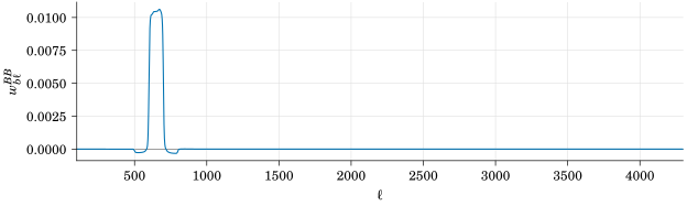
You can see some of the power is negative. That is, rather than being distributed as a \(\chi^2_\nu\) distribution, it is more like
\[\begin{align*} \mathcal{C}_{b , \text{eff.}} & \sim a \left( \chi^{2}_{\nu^{+}_{b}} - \chi^{2}_{\nu^{-}_{b}} \right) \\ \mathbb{E} \mathopen{} \left [ \mathcal{C}_{b , \text{eff.}} \right ] \mathclose{} & = C_{b} \Rightarrow a \equiv \frac{C_{b}}{\nu^{+}_{b} - \nu^{-}_{b}} \\ \operatorname{Var} \mathopen{} \left ( \mathcal{C}_{b , \text{eff.}} \right ) \mathclose{} & = a^{2} \left( 2 \nu^{+}_{b} + 2 \nu^{-}_{b} \right) = 2 C_{b}^{2} \frac{\nu^{+}_{b} + \nu^{-}_{b}}{\left( \nu^{+}_{b} - \nu^{-}_{b} \right)^{2}} \end{align*}\]
comparing this to eq. (28.1), we can define an effective d.o.f.
\[\nu_b^\text{eff} = \frac{(\nu^+ - \nu^-)^2}{\nu^+ + \nu^-}.\]
The new formula improves the agreement between MC error-bar and analytical error-bar, from \(\sim {10\,\%}\) to \(\sim {3\,\%}\) agreement for \(BB, EB, EE, TB, TE\) power-spectra, and from \(\sim {20\,\%}\) to \(\sim {13\,\%}\) agreement for \(TT\) power-spectrum19.
This improvement is crucial, as general agreement between the analytical error-bar and the MC error-bar is a good cross-check, and the likelihood used in sec. 28.3 contains \(ν\) which implicitly uses the analytical error-bar rather than the MC error-bar.
Error propagation & miscellaneous likelihood parameters
It is already mentioned that the likelihood is going to propagate the uncertainties of calibration parameters. Here we mention other sources of error.
As mentioned before, the filter transfer functions are estimated via 2 sets of 128 MC simulations, one without the \(B\)-mode signal, another without the \(E\)-mode signal. This results in a relative error in \(F_\ell\) peaked at \({1\,\%}\)-level in the low-\(\ell\) end. The final bin-width used is \(100\), making relative error of \(F_b\) to be at least an order of magnitude smaller.
Empirically, the agreement between the 2 sets of simulations above and the theory with BPWF is peaked at \(10^{-6}\)-level in the low-\(\ell\) end.
Because of these, and the fact that the statistical error from noise is much larger, errors from filter transfer function are negligible and will be ignored here.
Error from beam will be fitted similarly as in previous POLARBEAR \(B\)-mode publications, that is, an \(\ell\) dependent gain. The error-bar will be introduced in the likelihood equation automatically by having the following gain term,
\[a_i = a_{0, i} e^{-\frac{\ell (\ell +1) \sigma^2}{2}},\]
where \(σ\) is a free parameter in the likelihood.
Footnotes
“SELF-CALIBRATION OF COSMIC MICROWAVE BACKGROUND POLARIZATION EXPERIMENTS”.↩︎
Note that if we define absolute gain \(\beta\) in the TOD and hence the map, \(\alpha \equiv \beta^2\).↩︎
It will not be exactly uncorrelated in our case since we have far from a full sky map.↩︎
Note that this does not reduce statistical uncertainty in determining the absolute scale of the CMB polarizations per se. This is because there are other contributions to this absolute scale, such as the “absolute polarization efficiency”. If it can be shown that other kinds of systematics in determining this absolute scale are well controlled, then the benefits of getting a well-characterized absolute gain can result in meaningful reduction of statistical error in the CMB polarization measurements.↩︎
“A Measurement of the Cosmic Microwave Background B-Mode Polarization Power Spectrum at Sub-Degree Scales with POLARBEAR”.↩︎
See Technology (U.S.), NIST Handbook of Mathematical Functions Hardback and CD-ROM, , eq. 8.2.4.↩︎
“SciPy is a collection of mathematical algorithms and convenience functions built on the NumPy extension of Python.”↩︎
In other words, the PTE is a \(U[0, 1]\) random variable.↩︎
Consider the boolean flags as a time-series of boolean values where each indicates if a sub-scan is chosen to be in that null-split or not.↩︎
Minimum statistics is a special case of ordered statistics, where the CDF can be computed analytically given the original CDF if they are independent. In this case the original CDF is from a uniform discrete distribution of \(\frac{0, 1, \dots, 511}{512}\). It can be shown that it is skewed towards the left and more skewed as \(n_\text{family}\) increases.↩︎
Loosely speaking, it means it does not pass as easily.↩︎
Holm, “A Simple Sequentially Rejective Multiple Test Procedure”.↩︎
As we argued elsewhere we only have one observable universe that we cannot experiment on but to observe statistical properties from it.↩︎
“SELF-CALIBRATION OF COSMIC MICROWAVE BACKGROUND POLARIZATION EXPERIMENTS”.↩︎
“Likelihood Analysis of CMB Temperature and Polarization Power Spectra”.↩︎
“MASTER of the Cosmic Microwave Background Anisotropy Power Spectrum”.↩︎
The POLARBEAR Collaboration et al., “A Measurement of the Cosmic Microwave Background B-Mode Polarization Power Spectrum at Sub-Degree Scales with POLARBEAR”.↩︎
\(TT\) is not as i.i.d. as the others empirically, so the analytical model fails more here. See sec. 28.2.↩︎